In the realm of statistics and machine learning, understanding various probability distributions is paramount. One such fundamental distribution is the Binomial Distribution.
This distribution is not only a cornerstone in probability theory but also plays a crucial role in various machine learning algorithms and applications.
In this blog, we will delve into the concept of binomial distribution, its mathematical formulation, and its significance in the field of machine learning.
What is Binomial Distribution?
The binomial distribution is a discrete probability distribution that describes the number of successes in a fixed number of independent and identically distributed Bernoulli trials.
A Bernoulli trial is a random experiment where there are only two possible outcomes:
success (with probability ( p ))
failure (with probability ( 1 – p ))
Mathematical Formulation
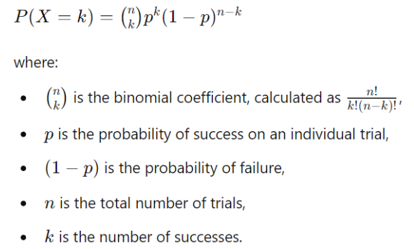
The probability of observing exactly k successes in n trials is given by the binomial probability formula:
Example 1: Tossing One Coin
Let’s start with a simple example of tossing a single coin.
Parameters
Number of trials (n) = 1
Probability of heads (p) = 0.5
Number of heads (k) = 1
Calculation
Binomial coefficient
Probability
So, the probability of getting exactly one head in one toss of a coin is 0.5 or 50%.
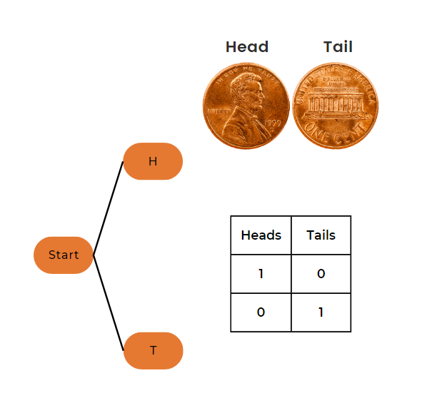
Example 2: Tossing Two Coins
Now, let’s consider the case of tossing two coins.
So, the probabilities for different numbers of heads in two-coin tosses are:
P(X = 0) = 0.25 – no heads
P(X = 1) = 0.5 – one head
P(X = 2) = 0.25 – two heads
Detailed Example: Predicting Machine Failure
Let’s consider a more practical example involving predictive maintenance in an industrial setting. Suppose we have a machine that is known to fail with a probability of 0.05 during a daily checkup. We want to determine the probability of the machine failing exactly 3 times in 20 days.
Step-by-Step Calculation
1. Identify Parameters
Number of trials (n) = 20 days
Probability of success (p) = 0.05 – failure is considered a success in this context
Number of successes (k) = 3 failures
2. Apply the Formula
3. Compute Binomial Coefficient
4. Calculate Probability
Plugging the values into the binomial formula
Substitute the values
P(X = 3) = 1140 × (0.05)3 × (0.95)17
Calculate (0.05)3
(0.05)3 = 0.000125
Calculate (0.95)17
(0.95)17 ≈ 0.411
5. Multiply all Components Together
P(X = 3) = 1140 × 0.000125 × 0.411 ≈ 0.0585
Therefore, the probability of the machine failing exactly 3 times in 20 days is approximately 0.0585 or 5.85%.
Role of Binomial Distribution in Machine Learning
The binomial distribution is integral to several aspects of machine learning, providing a foundation for understanding and modeling binary events, hypothesis testing, and beyond.
Let’s explore how it intersects with various machine-learning concepts and techniques.
Binary Classification
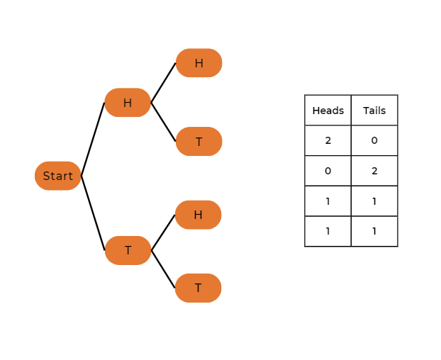
In binary classification problems, where the outcomes are often categorized as success or failure, the binomial distribution forms the underlying probabilistic model. For instance, if we are predicting whether an email is spam or not, each email can be thought of as a Bernoulli trial.
Algorithms like Logistic Regression and Support Vector Machines (SVM) are particularly designed to handle these binary outcomes.
An example of binary classification – ResearchGate
Understanding the binomial distribution helps in correctly interpreting the results of these classifiers. The performance metrics such as accuracy, precision, recall, and F1-score ultimately derive from the binomial probability model.
This understanding ensures that we can make informed decisions about model improvements and performance evaluation.
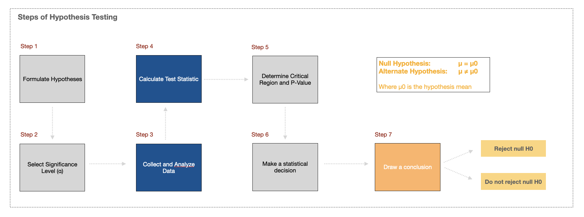
Hypothesis Testing
Statistical hypothesis testing, essential in validating machine learning models, often employs the binomial distribution to ascertain the significance of observed outcomes.
A typical process of hypothesis testing – Source: LinkedIn
For instance, in A/B testing, which is widely used in machine learning for comparing model performance or feature impact, the binomial distribution helps in calculating p-values and confidence intervals.
Consider an example where we want to determine if a new feature in a recommendation system improves user click-through rates. By modeling the click events as a binomial distribution, we can perform a hypothesis test to evaluate if the observed improvement is statistically significant or just due to random chance.
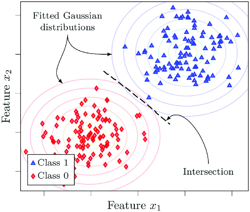
Generative Models
Generative models such as Naive Bayes leverage binomial distributions to model the probability of observing certain classes given specific features. This is particularly useful when dealing with binary or categorical data.
An illustration of Naive Bayes classifier – Source: ResearchGate
In text classification tasks, for example, the presence or absence of certain words (features) in a document can be modeled using binomial distributions to predict the document’s category (class).
By understanding the binomial distribution, we can better grasp how these models work under the hood, leading to more effective feature engineering and model tuning.
Monte Carlo simulations, which are used in various machine learning applications for uncertainty estimation and decision-making, often rely on binomial distributions to model and simulate binary events over numerous trials.
These simulations can help in understanding the variability and uncertainty in model predictions, providing a robust framework for decision-making in the presence of randomness.
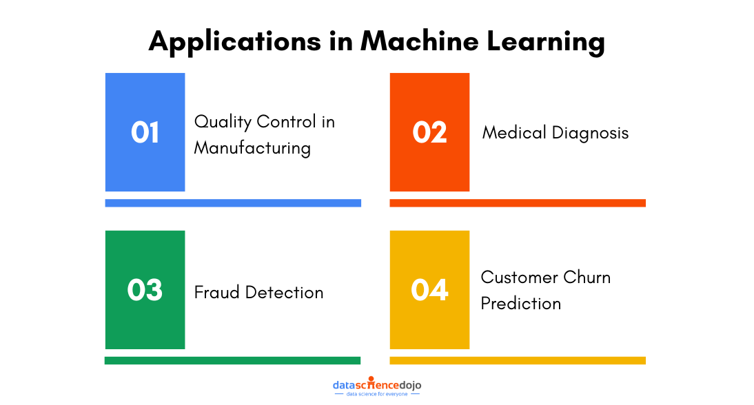
Practical Applications in Machine Learning
Quality Control in Manufacturing
In manufacturing, maintaining high-quality standards is crucial. Machine learning models are often deployed to predict the likelihood of defects in products.
Here, the binomial distribution is used to model the number of defective items in a batch. By understanding the distribution, we can set appropriate thresholds and confidence intervals to decide when to take corrective actions.
In medical diagnosis, machine learning models assist in predicting the presence or absence of a disease based on patient data. The binomial distribution provides a framework for understanding the probabilities of correct and incorrect diagnoses.
This is critical for evaluating the performance of diagnostic models and ensuring they meet the necessary accuracy and reliability standards.
Fraud Detection
Fraud detection systems in finance and e-commerce rely heavily on binary classification models to distinguish between legitimate and fraudulent transactions. The binomial distribution aids in modeling the occurrence of fraud and helps in setting detection thresholds that balance false positives and false negatives effectively.
Predicting customer churn is vital for businesses to retain their customer base. Machine learning models predict whether a customer will leave (churn) or stay (retain). The binomial distribution helps in understanding the probabilities of churn events and in setting up retention strategies based on these probabilities.
Why Use Binomial Distribution?
Binomial distribution is a fundamental concept that finds extensive application in machine learning. From binary classification to hypothesis testing and generative models, understanding and leveraging this distribution can significantly enhance the performance and interpretability of machine learning models.
By mastering the binomial distribution, you equip yourself with a powerful tool for tackling a wide range of problems in statistics and machine learning.
Feel free to dive deeper into this topic, experiment with different values, and explore the fascinating world of probability distributions in machine learning!
Machine learning (ML) is a field where both art and science converge to create models that can predict outcomes based on data. One of the most effective strategies employed in ML to enhance model performance is ensemble methods.
Rather than relying on a single model, ensemble methods combine multiple models to produce better results. This approach can significantly boost accuracy, reduce overfitting, and improve generalization.
In this blog, we’ll explore various ensemble techniques, their working principles, and their applications in real-world scenarios.
What Are Ensemble Methods?
Ensemble methods are techniques that create multiple models and then combine them to produce a more accurate and robust final prediction. The idea is that by aggregating the predictions of several base models, the ensemble can capture the strengths of each individual model while mitigating their weaknesses.
Ensemble methods are used to improve the robustness and generalization of machine learning models by combining the predictions of multiple models. This can reduce overfitting and improve performance on unseen data.
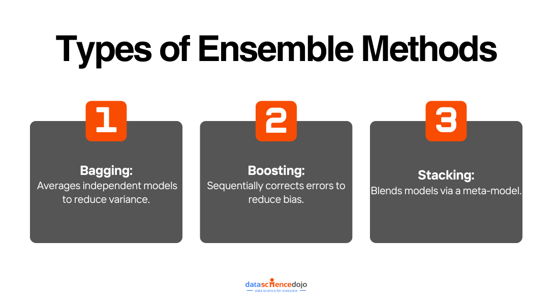
There are three primary types of ensemble methods: Bagging, Boosting, and Stacking.
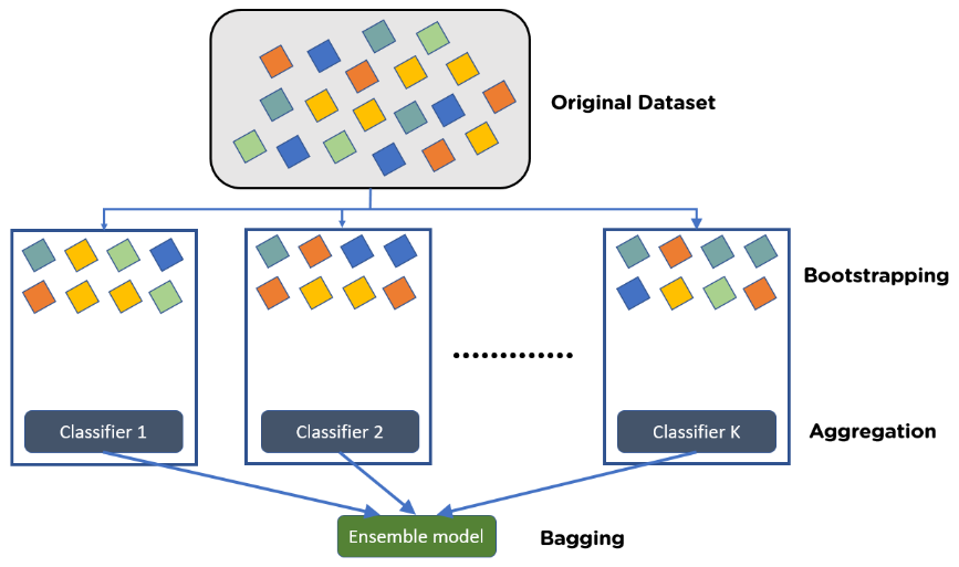
Bagging (Bootstrap Aggregating)
Bagging involves creating multiple subsets of the original dataset using bootstrap sampling (random sampling with replacement). Each subset is used to train a different model, typically of the same type, such as decision trees. The final prediction is made by averaging (for regression) or voting (for classification) the predictions of all models.
An outlook of bagging – Source: LinkedIn
How Bagging Works:
Bootstrap Sampling: Create multiple subsets from the original dataset by sampling with replacement.
Model Training: Train a separate model on each subset.
Aggregation: Combine the predictions of all models by averaging (regression) or majority voting (classification).
Random Forest
Random Forest is a popular bagging method where multiple decision trees are trained on different subsets of the data, and their predictions are averaged to get the final result.
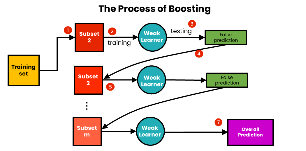
Boosting
Boosting is a sequential ensemble method where models are trained one after another, each new model focusing on the errors made by the previous models. The final prediction is a weighted sum of the individual model’s predictions.
A representation of boosting – Source: Medium
How Boosting Works:
Initialize Weights: Start with equal weights for all data points.
Sequential Training: Train a model and adjust weights to focus more on misclassified instances.
Aggregation: Combine the predictions of all models using a weighted sum.
AdaBoost (Adaptive Boosting)
It assigns weights to each instance, with higher weights given to misclassified instances. Subsequent models focus on these hard-to-predict instances, gradually improving the overall performance.
It builds models sequentially, where each new model tries to minimize the residual errors of the combined ensemble of previous models using gradient descent.
XGBoost (Extreme Gradient Boosting)
An optimized version of Gradient Boosting, known for its speed and performance, is often used in competitions and real-world applications.
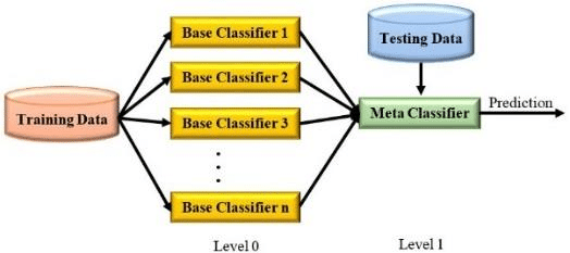
Stacking
Stacking, or stacked generalization, involves training multiple base models and then using their predictions as inputs to a higher-level meta-model. This meta-model is responsible for making the final prediction.
Visual concept of stacking – Source: ResearchGate
How Stacking Works:
Base Model Training: Train multiple base models on the training data.
Meta-Model Training: Use the predictions of the base models as features to train a meta-model.
Example:
A typical stacking ensemble might use logistic regression as the meta-model and decision trees, SVMs, and KNNs as base models.
Benefits of Ensemble Methods
Improved Accuracy
By combining multiple models, ensemble methods can significantly enhance prediction accuracy.
Robustness
Ensemble models are less sensitive to the peculiarities of a particular dataset, making them more robust and reliable.
Reduction of Overfitting
By averaging the predictions of multiple models, ensemble methods reduce the risk of overfitting, especially in high-variance models like decision trees.
Versatility
Ensemble methods can be applied to various types of data and problems, from classification to regression tasks.
Applications of Ensemble Methods
Ensemble methods have been successfully applied in various domains, including:
Healthcare: Improving the accuracy of disease diagnosis by combining different predictive models.
Finance: Enhancing stock price prediction by aggregating multiple financial models.
Computer Vision: Boosting the performance of image classification tasks with ensembles of CNNs.
Now let’s walk through the implementation of a Random Forest classifier in Python using the popular scikit-learn library. We’ll use the Iris dataset, a well-known dataset in the machine learning community, to demonstrate the steps involved in training and evaluating a Random Forest model.
Explanation of the Code
Import Necessary Libraries
We start by importing the necessary libraries. numpy is used for numerical operations, train_test_split for splitting the dataset, RandomForestClassifier for building the model, accuracy_score for evaluating the model, and load_iris to load the Iris dataset.
Load the Iris Dataset
The Iris dataset is loaded using load_iris(). The dataset contains four features (sepal length, sepal width, petal length, and petal width) and three classes (Iris setosa, Iris versicolor, and Iris virginica).
Split the Dataset
We split the dataset into training and testing sets using train_test_split(). Here, 30% of the data is used for testing, and the rest is used for training. The random_state parameter ensures the reproducibility of the results.
Initialize the RandomForestClassifier
We create an instance of the RandomForestClassifier with 100 decision trees (n_estimators=100). The random_state parameter ensures that the results are reproducible.
Train the Model
We train the Random Forest classifier on the training data using the fit() method.
Make Predictions
After training, we use the predict() method to make predictions on the testing data.
Evaluate the Model
Finally, we evaluate the model’s performance by calculating the accuracy using the accuracy_score() function. The accuracy score is printed to two decimal places.
Output Analysis
When you run this code, you should see an output similar to:
This output indicates that the Random Forest classifier achieved 100% accuracy on the testing set. This high accuracy is expected for the Iris dataset, as it is relatively small and simple, making it easy for many models to achieve perfect or near-perfect performance.
In practice, the accuracy may vary depending on the complexity and nature of the dataset, but Random Forests are generally robust and reliable classifiers.
By following this guided practice, you can see how straightforward it is to implement a Random Forest model in Python. This powerful ensemble method can be applied to various datasets and problems, offering significant improvements in predictive performance.
Summing it Up
To sum up, Ensemble methods are powerful tools in the machine learning toolkit, offering significant improvements in predictive performance and robustness. By understanding and applying techniques like bagging, boosting, and stacking, you can create models that are more accurate and reliable.
Ensemble methods are not just theoretical constructs; they have practical applications in various fields. By leveraging the strengths of multiple models, you can tackle complex problems with greater confidence and precision.
By understanding machine learning algorithms, you can appreciate the power of this technology and how it’s changing the world around you! It’s like having a super-powered tool to sort through information and make better sense of the world.
So, just like a super sorting system for your toys, machine learning algorithms can help you organize and understand massive amounts of data in many ways:
Recommend movies you might like by learning what kind of movies you watch already.
Spot suspicious activity on your credit card by learning what your normal spending patterns look like.
Help doctors diagnose diseases by analyzing medical scans and patient data.
Predict traffic jams by learning patterns in historical traffic data.
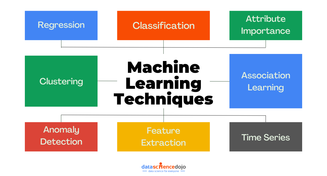
Key Machine Learning Techniques
1. Regression
Regression, much like predicting how much popcorn you need for movie night, is a cornerstone of machine learning. It delves into the realm of continuous predictions, where the target variable you’re trying to estimate takes on numerical values. Let’s unravel the technicalities behind this technique:
Regression algorithms learn from labeled data, similar to classification. However, in this case, the labels are continuous values. For example, you might have data on house size (features) and their corresponding sale prices (target variable).
The algorithm’s goal is to uncover the underlying relationship between the features and the target variable. This relationship is often depicted by a mathematical function (like a line or curve).
Once trained, the model can predict the target variable for new, unseen data points based on their features.
Types of Regression Problems:
Linear Regression: This is the simplest and most common form, where the relationship between features and the target variable is modeled by a straight line.
Polynomial Regression: When the linear relationship doesn’t suffice, polynomials (curved lines) are used to capture more complex relationships.
Non-linear Regression: There’s a vast array of non-linear models (e.g., decision trees, support vector regression) that can model even more intricate relationships between features and the target variable.
Technical Considerations:
Feature Engineering: As with classification, selecting and potentially transforming features significantly impacts model performance.
Evaluating Model Fit: Metrics, like mean squared error (MSE) or R-squared, are used to assess how well the model’s predictions align with the actual target values.
Overfitting and Underfitting: Similar to classification, achieving a balance between model complexity and generalizability is crucial. Techniques like regularization can help prevent overfitting.
Residual Analysis: Examining the residuals (differences between predicted and actual values) can reveal underlying patterns and potential issues with the model.
Real-world Applications:
Regression finds applications in various domains:
Weather Forecasting: Predicting future temperatures based on historical data and current conditions.
Stock Market Analysis: Forecasting future stock prices based on historical trends and market indicators.
Sales Prediction: Estimating future sales figures based on past sales data and marketing campaigns.
Customer Lifetime Value (CLV) Prediction: Forecasting the total revenue a customer will generate over their relationship with a company.
Technical Nuances:
While linear regression offers a good starting point, understanding advanced regression techniques allows you to model more complex relationships and create more accurate predictions in diverse scenarios.
Additionally, addressing issues like multi-collinearity (correlated features) and hetero-scedasticity (unequal variance of errors) becomes crucial as regression models become more sophisticated.
By comprehending these technical aspects, you gain a deeper understanding of how regression algorithms unveil the hidden patterns within your data, enabling you to make informed predictions and solve real-world problems.
Classification algorithms learn from labeled data. This means each data point has a pre-defined category or class label attached to it. For example, in spam filtering, emails might be labeled as “spam” or “not-spam.”
It analyzes the features or attributes of the data (like word content in emails or image pixels in pictures).
Based on this analysis, it builds a model that can predict the class label for new, unseen data points.
Types of Classification Problems:
Binary Classification: This is the simplest case, where there are only two possible categories (spam/not-spam, cat/dog).
Multi-Class Classification: Here, there are more than two categories (e.g., classifying handwritten digits into 0, 1, 2, …, 9).
Multi-Label Classification: A data point can belong to multiple classes simultaneously (e.g., an image might contain both a cat and a dog).
Common Classification Algorithms:
Logistic Regression: A popular choice for binary classification, it uses a mathematical function to model the probability of a data point belonging to a particular class.
Support Vector Machines (SVM): This algorithm finds a hyperplane that best separates data points of different classes in high-dimensional space.
Decision Trees: These work by asking a series of yes/no questions based on data features to classify data points.
K-Nearest Neighbors (KNN): This method classifies a data point based on the majority class of its K nearest neighbors in the training data.
Learn how machine learning will revolutionize demand planning
Technical aspects to consider:
Feature Engineering: Choosing the right features and potentially transforming them (e.g., converting text to numerical features) is crucial for model performance.
Overfitting and Underfitting: The model should neither be too specific to the training data (overfitting) nor too general (underfitting). Techniques like regularization can help balance this.
Evaluation Metrics: Performance is measured using metrics like accuracy, precision, recall, and F1-score, depending on the specific classification task.
Real-world Applications:
Classification is used extensively across various domains:
Fraud Detection: Identifying suspicious transactions on credit cards.
Medical Diagnosis: Classifying medical images or predicting disease risk factors.
Sentiment Analysis: Classifying text data as positive, negative, or neutral sentiment.
3. Attribute Importance
Just like understanding which features matter most when sorting your laundry, delves into the significance of individual features within your machine-learning model. Here’s a breakdown of the technicalities.
Machine learning models utilize various features (attributes) from your data to make predictions. Not all features, however, contribute equally. Attribute importance helps you quantify the relative influence of each feature on the model’s predictions.
Technical Approaches:
There are several techniques to assess attribute importance, each with its own strengths and weaknesses:
Feature Permutation: This method randomly shuffles the values of a single feature and observes the resulting change in model performance. A significant drop suggests that feature is important.
Feature Impurity Measures: This approach, commonly used in decision trees, calculates the average decrease in impurity (e.g., Gini index) when a split is made on a particular feature. Higher impurity reduction indicates greater importance.
Model-Specific Techniques: Some models have built-in methods for calculating attribute importance. For example, Random Forests track the improvement in prediction accuracy when features are included in splits.
Benefits of Understanding Attribute Importance:
Model Interpretability: By knowing which features are most important, you gain insights into how the model arrives at its predictions. This is crucial for understanding model behavior and building trust.
Feature Selection: Identifying irrelevant or redundant features allows you to streamline your data and potentially improve model performance by focusing on the most impactful features.
Domain Knowledge Integration: Attribute importance can highlight features that align with your domain expertise, validating the model’s reasoning or prompting further investigation.
Technical Considerations:
Choice of Technique: The most suitable method depends on the model you’re using and the type of data you have. Experimenting with different approaches may be necessary.
Normalization: The importance scores might need normalization across features for better comparison, especially when features have different scales.
Limitations: Importance scores can be influenced by interactions between features. A seemingly unimportant feature might play a crucial role in conjunction with others.
Real-world Applications:
Attribute importance finds applications in various domains:
Fraud Detection: Identifying the financial factors (e.g., transaction amount, location) that most influence fraud prediction allows for targeted risk mitigation strategies.
Medical Diagnosis: Understanding which symptoms are most crucial for disease prediction helps healthcare professionals prioritize tests and interventions.
Customer Churn Prediction: Knowing which customer attributes (e.g., purchase history, demographics) are most indicative of churn allows businesses to develop targeted retention strategies.
By understanding attribute importance, you gain valuable insights into the inner workings of your machine-learning models. This empowers you to make informed decisions about feature selection, improve model interpretability, and ultimately, achieve better performance.
4. Association Learning
Akin to noticing your friend always buying peanut butter with jelly, is a technique in machine learning that uncovers hidden relationships between different features (attributes) within your data. Let’s delve into the technical aspects:
The Core Concept:
Association learning algorithms analyze large datasets to discover frequent patterns of co-occurrence between features. These patterns are often expressed as association rules, which take the form “if A, then B with confidence X%”. Here’s an example:
Rule: If a customer buys diapers (A), then they are also likely to buy wipes (B) with 80% confidence (X%).
Technical Approaches:
Apriori Algorithm: This is a foundational algorithm that employs a breadth-first search to identify frequent itemsets (groups of features that appear together frequently). These itemsets are then used to generate association rules with a minimum support (frequency) and confidence (correlation) threshold.
FP-Growth Algorithm: This is an optimization over Apriori that uses a frequent pattern tree structure to efficiently mine frequent itemsets, reducing the number of candidate rules generated.
Benefits of Association Learning:
Market Basket Analysis: Understanding buying patterns helps retailers recommend complementary products and optimize product placement in stores.
Customer Segmentation: Identifying groups of customers with similar purchasing behavior enables targeted marketing campaigns.
Fraud Detection: Discovering unusual co-occurrences in transactions can help identify potential fraudulent activities.
Technical Considerations:
Minimum Support and Confidence: Setting appropriate thresholds for both is crucial. A high support ensures the rule is not based on rare occurrences, while a high confidence guarantees a strong correlation between features.
Data Sparsity: Association learning often works best with large, dense datasets. Sparse data with many infrequent features can lead to unreliable results.
Lift: This metric goes beyond confidence and considers the baseline probability of feature B appearing independently. A lift value greater than 1 indicates a stronger association than random chance.
Real-world Applications:
Association learning finds applications in various domains:
Recommendation Systems: Online platforms leverage association rules to recommend products or content based on a user’s past purchases or browsing behavior.
Clickstream Analysis: Understanding how users navigate websites through association rules helps optimize website design and user experience.
Network Intrusion Detection: Identifying unusual patterns in network traffic can help detect potential security threats.
By understanding the technicalities of association learning, you can unlock valuable insights hidden within your data. These insights enable you to make informed decisions in areas like marketing, fraud prevention, and recommendation systems.
Time series data, like your daily steps or stock prices, unfolds over time. Machine learning unlocks the secrets within this data by analyzing its temporal patterns. Let’s delve into the technicalities of time series analysis:
The Core Idea:
Time series data consists of data points collected at uniform time intervals. These data points represent the value of a variable at a specific point in time.
Time series analysis focuses on modeling and understanding the trends, seasonality, and cyclical patterns within this data.
Machine learning algorithms can then be used to forecast future values based on historical data and the underlying patterns.
Technical Approaches:
There are various models and techniques used for time series analysis:
Moving Average Models: These models take the average of past data points to predict future values. They are simple but effective for capturing short-term trends.
Exponential Smoothing: This builds on moving averages by giving more weight to recent data points, and adapting to changing trends.
ARIMA (Autoregressive Integrated Moving Average): This is a powerful statistical model that captures autoregression (past values influencing future values) and seasonality.
Recurrent Neural Networks (RNNs): These powerful deep learning models can learn complex patterns and long-term dependencies within time series data, making them suitable for more intricate forecasting tasks.
Stationarity: Many time series models assume the data is stationary, meaning the statistical properties (mean, variance) don’t change over time. Differencing techniques might be necessary to achieve stationarity.
Feature Engineering: Creating new features based on existing time series data (e.g., lags, rolling averages) can improve model performance.
Evaluation Metrics: Metrics like Mean Squared Error (MSE) or Mean Absolute Error (MAE) are used to assess the accuracy of forecasts generated by the model.
Real-world Applications:
Time series analysis finds applications in various domains:
Supply Chain Management: Forecasting demand for products to optimize inventory management.
Sales Forecasting: Predicting future sales figures to plan production and marketing strategies.
Weather Forecasting: Predicting future temperatures, precipitation, and other weather patterns.
By understanding the technicalities of time series analysis, you can unlock the power of time-based data for forecasting and making informed decisions in various domains. Machine learning offers sophisticated tools for extracting valuable insights from the ever-flowing stream of time series data.
Feature extraction, akin to summarizing a movie by its genre, actors, and director, plays a crucial role in machine learning. It involves transforming raw data into a more meaningful and informative representation for machine learning models to work with. Let’s delve into the technical aspects:
The Core Idea:
Raw data can be complex and high-dimensional. Machine learning models often struggle to process and learn from this raw data directly.
Feature extraction aims to extract a smaller set of features from the raw data that are more relevant to the machine-learning task at hand. These features capture the essential information needed for the model to make predictions.
Technical Approaches:
There are various techniques for feature extraction, depending on the type of data you’re dealing with:
Feature Selection: This involves selecting a subset of existing features that are most informative and relevant to the prediction task. Techniques like correlation analysis and filter methods can be used for this purpose.
Dimensionality Reduction: Techniques like Principal Component Analysis (PCA) project high-dimensional data onto a lower-dimensional space while preserving most of the information. This reduces the complexity of the data and improves model efficiency.
Feature Engineering: This involves creating entirely new features from the existing data. This can be done through domain knowledge, mathematical transformations, or feature combinations. For example, creating new features like “day of the week” from a date column.
Benefits of Feature Extraction:
Improved Model Performance: By focusing on relevant features, the model can learn more effectively and make better predictions.
Reduced Training Time: Lower dimensional data allows for faster training of machine learning models.
Reduced Overfitting: Feature extraction can help prevent overfitting by reducing the number of features the model needs to learn from.
Technical Considerations:
Choosing the Right Technique: The best approach depends on the type of data and the machine learning task. Experimentation with different techniques might be necessary.
Domain Knowledge: Feature engineering often relies on your domain expertise to create meaningful features from the raw data.
Evaluation and Interpretation: It’s essential to evaluate the impact of feature extraction on model performance. Additionally, understanding the extracted features can provide insights into the model’s behavior.
Real-world Applications:
Feature extraction finds applications in various domains:
Image Recognition: Extracting features like edges, shapes, and colors from images helps models recognize objects.
Text Analysis: Feature extraction might involve extracting keywords, sentiment scores, or topic information from text data for tasks like sentiment analysis or document classification.
Sensor Data Analysis: Extracting relevant features from sensor data (e.g., temperature, pressure) helps models monitor equipment health or predict system failures.
By understanding the intricacies of feature extraction, you can transform raw data into a goldmine of information for your machine learning models. This empowers you to extract the essence of your data and unlock its full potential for accurate predictions and insightful analysis.
7. Anomaly Detection
Anomaly detection, like noticing a misspelled word in an essay, equips machine learning models to identify data points that deviate significantly from the norm. These anomalies can signal potential errors, fraud, or critical events that require attention. Let’s delve into the technical aspects:
The Core Idea:
Machine learning models learn the typical patterns and characteristics of data during the training phase.
Anomaly detection algorithms leverage this knowledge to identify data points that fall outside the expected range or exhibit unusual patterns.
Technical Approaches:
There are several approaches to anomaly detection, each suitable for different scenarios:
Statistical Methods: Techniques like outlier detection using standard deviation or z-scores can identify data points that statistically differ from the majority.
Distance-based Methods: These methods measure the distance of a data point from its nearest neighbors in the feature space. Points far away from others are considered anomalies.
Clustering Algorithms: Clustering algorithms can group data points with similar features. Points that don’t belong to any well-defined cluster might be anomalies.
Machine Learning Models: Techniques like One-Class Support Vector Machines (OCSVM) learn a model of “normal” data and then flag any points that deviate from this model as anomalies.
Technical Considerations:
Defining Normality: Clearly defining what constitutes “normal” data is crucial for effective anomaly detection. This often relies on historical data and domain knowledge.
False Positives and False Negatives: Anomaly detection algorithms can generate false positives (flagging normal data as anomalies) and false negatives (missing actual anomalies). Balancing these trade-offs is essential.
Threshold Selection: Setting appropriate thresholds for anomaly scores determines how sensitive the system is to detecting anomalies. A high threshold might miss critical events, while a low threshold can lead to many false positives.
Real-world Applications:
Anomaly detection finds applications in various domains:
Fraud Detection: Identifying unusual transactions in credit card usage patterns can help prevent fraudulent activities.
Network Intrusion Detection: Detecting anomalies in network traffic patterns can help identify potential cyberattacks.
Equipment Health Monitoring: Identifying anomalies in sensor data from machines can predict equipment failures and prevent costly downtime.
Medical Diagnosis: Detecting anomalies in medical scans or patient vitals can help diagnose potential health problems.
By understanding the technicalities of anomaly detection, you can equip your machine learning models with the ability to identify the unexpected. This proactive approach allows you to catch issues early on, improve system security, and optimize various processes across diverse domains.
8. Clustering
Clustering, much like grouping similar-colored socks together, is a powerful unsupervised machine learning technique. It delves into the world of unlabeled data, where data points lack predefined categories.
Clustering algorithms automatically group data points with similar characteristics, forming meaningful clusters. Let’s explore the technical aspects:
The Core Idea:
Unsupervised learning means the data points don’t have pre-assigned labels (e.g., shirt, pants).
Clustering algorithms analyze the features (attributes) of data points and group them based on their similarity.
The similarity between data points is often measured using distance metrics like Euclidean distance (straight line distance) in a multi-dimensional feature space.
Types of Clustering Algorithms:
K-Means Clustering: This is a popular and efficient algorithm that partitions data points into a predefined number of clusters (k). It iteratively calculates the centroid (center) of each cluster and assigns data points to the closest centroid until convergence (stable clusters).
Hierarchical Clustering: This method builds a hierarchy of clusters, either in a top-down (divisive) fashion by splitting large clusters or a bottom-up (agglomerative) fashion by merging smaller clusters. The level of granularity in the hierarchy determines the final clustering results.
Density-Based Spatial Clustering of Applications with Noise (DBSCAN): This approach identifies clusters based on areas of high data point density, separated by areas of low density (noise). It doesn’t require predefining the number of clusters and can handle outliers effectively.
Technical Considerations:
Choosing the Right Algorithm: The optimal algorithm depends on the nature of your data, the desired number of clusters, and the presence of noise. Experimentation might be necessary.
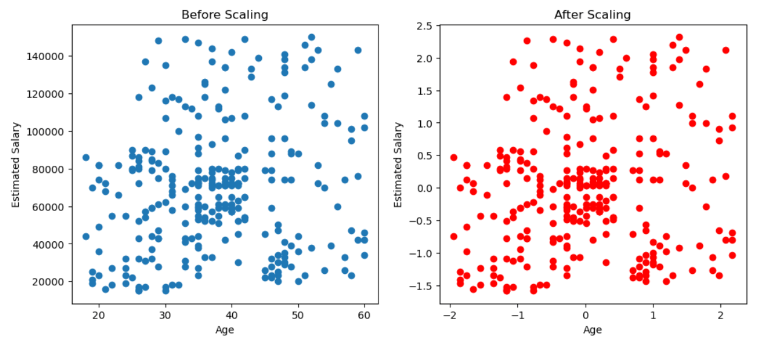
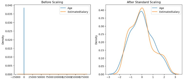
Data Preprocessing: Feature scaling and normalization might be crucial for ensuring all features contribute equally to the distance calculations used in clustering.
Evaluating Clustering Results: Metrics like silhouette score or Calinski-Harabasz index can help assess the quality and separation between clusters, but domain knowledge is also valuable for interpreting the results.
Real-world Applications:
Clustering finds applications in various domains:
Customer Segmentation: Grouping customers with similar purchasing behavior allows for targeted marketing campaigns and loyalty programs.
Image Segmentation: Identifying objects or regions of interest within images by grouping pixels with similar color or texture.
Document Clustering: Grouping documents based on topic or content for efficient information retrieval.
Social Network Analysis: Identifying communities or groups of users with similar interests or connections.
By understanding the machine learning technique of clustering, you gain the ability to uncover hidden patterns within your unlabeled data. This allows you to segment data for further analysis, discover new customer groups, and gain valuable insights into the structure of your data.
Kickstart your Learning Journey Today!
In summary, learning machine learning algorithms equips you with valuable skills, opens up career opportunities, and empowers you to make a significant impact in today’s data-driven world. Whether you’re a student, professional, or entrepreneur, investing in ML knowledge can enhance your career prospects.
In the ever-evolving landscape of artificial intelligence (AI), staying informed about the latest advancements, tools, and trends can often feel overwhelming. This is where AI newsletters come into play, offering a curated, digestible format that brings you the most pertinent updates directly to your inbox.
Learn to create a bird recognition app using Microsoft Custom Vision AI and Power BI
Whether you are an AI professional, a business leader leveraging AI technologies, or simply an enthusiast keen on understanding AI’s societal impact, subscribing to the right newsletters can make all the difference. In this blog, we delve into the 6 best AI newsletters of 2024, each uniquely tailored to keep you ahead of the curve.
From deep dives into machine learning research to practical guides on integrating AI into your daily workflow, these newsletters offer a wealth of knowledge and insights.
Join us as we explore the top AI newsletters that will help you navigate the dynamic world of artificial intelligence with ease and confidence.
What are AI Newsletters?
AI newsletters are curated publications that provide updates, insights, and analyses on various topics related to artificial intelligence (AI). They serve as a valuable resource for staying informed about the latest developments, research breakthroughs, ethical considerations, and practical applications of AI.
These newsletters cater to different audiences, including AI professionals, business leaders, researchers, and enthusiasts, offering content in a digestible format.
The primary benefits of subscribing to AI newsletters include:
Consolidation of Information: AI newsletters aggregate the most important news, articles, research papers, and resources from a variety of sources, providing readers with a comprehensive update in a single place.
Curation and Relevance: Editors typically curate content based on its relevance, novelty, and impact, ensuring that readers receive the most pertinent updates without being overwhelmed by the sheer volume of information.
Regular Updates: These newsletters are typically delivered on a regular schedule (daily, weekly, or monthly), ensuring that readers are consistently updated on the latest AI developments.
Expert Insights: Many AI newsletters are curated by experts in the field, providing additional commentary, insights, or summaries that help readers understand complex topics.
Accessible Learning: For individuals new to the field or those without a deep technical background, newsletters offer an accessible way to learn about AI, often presenting information clearly and linking to additional resources for deeper learning.
Community Building: Some newsletters allow for reader engagement and interaction, fostering a sense of community among readers and providing networking and learning opportunities from others in the field.
Career Advancement: For professionals, staying updated on the latest AI developments can be critical for career development. Newsletters may also highlight job openings, events, courses, and other opportunities.
Overall, AI newsletters are an essential tool for anyone looking to stay informed and ahead in the fast-paced world of artificial intelligence. Let’s look at the best AI newsletters you must follow in 2024 for the latest updates and trends in AI.
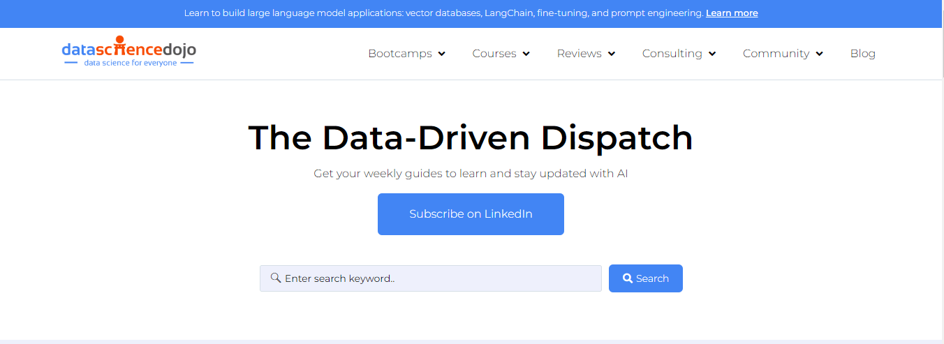
1. Data-Driven Dispatch
Data-Driven Dispatch
Over 100,000 subscribers
Data-Driven Dispatch is a weekly newsletter by Data Science Dojo. It focuses on a wide range of topics and discussions around generative AI and data science. The newsletter aims to provide comprehensive guidance, ensuring the readers fully understand the various aspects of AI and data science concepts.
To ensure proper discussion, the newsletter is divided into 5 sections:
AI News Wrap: Discuss the latest developments and research in generative AI, data science, and LLMs, providing up-to-date information from both industry and academia.
The Must Read: Provides insightful resource picks like research papers, articles, guides, and more to build your knowledge in the topics of your interest within AI, data science, and LLM.
Professional Playtime: Looks at technical topics from a fun lens of memes, jokes, engaging quizzes, and riddles to stimulate your creativity.
Hear it From an Expert: Includes important global discussions like tutorials, podcasts, and live-session recommendations on generative AI and data science.
Career Development Corner: Shares recommendations for top-notch courses and boot camps as resources to boost your career progression.
Target Audience
It caters to a wide and diverse audience, including engineers, data scientists, the general public, and other professionals. The diversity of its content ensures that each segment of individuals gets useful and engaging information.
Thus, Data-Driven Dispatch is an insightful and useful resource among modern newsletters to provide useful information and initiate comprehensive discussions around concepts of generative AI, data science, and LLMs.
2. ByteByteGo
ByteByteGo
Over 500,000 subscribers
The ByteByteGo Newsletter is a well-regarded publication that aims to simplify complex systems into easily understandable terms. It is authored by Alex Xu, Sahn Lam, and Hua Li, who are also known for their best-selling system design book series.
The newsletter provides insights into system design and technical knowledge. It is aimed at software engineers and tech enthusiasts who want to stay ahead in the field by providing in-depth insights into software engineering and technology trends
Target Audience
Software engineers, tech enthusiasts, and professionals looking to improve their skills in system design, cloud computing, and scalable architectures. Suitable for both beginners and experienced professionals.
Subscription Options
It is a weekly newsletter with a range of subscription options. The choices are listed below:
The weekly issue is released on Saturday for free subscribers
A weekly issue on Saturday, deep dives on Wednesdays, and a chance for topic suggestions for premium members
Group subscription at reduced rates is available for teams
Purchasing power parities are available for residents of countries with low purchasing power
Thus, ByteByteGo is a promising platform with a multitude of subscription options for your benefit. The newsletter is praised for its ability to break down complex technical topics into simpler terms, making it a valuable resource for those interested in system design and technical growth.
3. The Rundown AI
The Rundown AI
Over 600,000 subscribers
The Rundown AI is a daily newsletter by Rowan Cheung offering a comprehensive overview of the latest developments in the field of artificial intelligence (AI). It is a popular source for staying up-to-date on the latest advancements and discussions.
The newsletter has two distinct divisions:
Rundown AI: This section is tailored for those wanting to stay updated on the evolving AI industry. It provides insights into AI applications and tutorials to enhance knowledge in the field.
Rundown Tech: This section delivers updates on breakthrough developments and new products in the broader tech industry. It also includes commentary and opinions from industry experts and thought leaders.
Target Audience
The Rundown AI caters to a broad audience, including both industry professionals (e.g., researchers, and developers) and enthusiasts who want to understand AI’s growing impact.
There are no paid options available. You can simply subscribe to the newsletter for free from the website. Overall, The Rundown AI stands out for its concise and structured approach to delivering daily AI news, making it a valuable resource for both novices and experts in the AI industry.
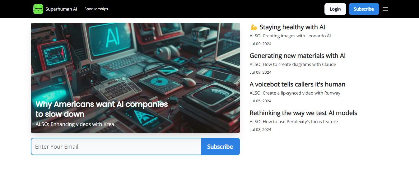
4. Superhuman AI
Superhuman AI
Over 700,000 subscribers
The Superhuman AI is a daily AI-focused newsletter curated by Zain Kahn. It is specifically focused on discussions around boosting productivity and leveraging AI for professional success. Hence, it caters to individuals who want to work smarter and achieve more in their careers.
The newsletter also includes tutorials, expert interviews, business use cases, and additional resources to help readers understand and utilize AI effectively. With its easy-to-understand language, it covers all the latest AI advancements in various industries like technology, art, and sports.
It is free and easily accessible to anyone who is interested. You can simply subscribe to the newsletter by adding your email to their mailing list on their website.
Target Audience
The content is tailored to be easily digestible even for those new to the field, providing a summarized format that makes complex topics accessible. It also targets professionals who want to optimize their workflows. It can include entrepreneurs, executives, knowledge workers, and anyone who relies on integrating AI into their work.
It can be concluded that the Superhuman newsletter is an excellent resource for anyone looking to stay informed about the latest developments in AI, offering a blend of practical advice, industry news, and engaging content.
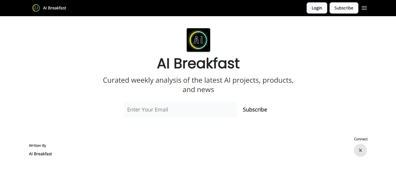
5. AI Breakfast
AI Breakfast
54,000 subscribers
The AI Breakfast newsletter is designed to provide readers with a comprehensive yet easily digestible summary of the latest developments in the field of AI. It publishes weekly, focusing on in-depth AI analysis and its global impact. It tends to support its claims with relevant news stories and research papers.
Hence, it is a credible source for people who want to stay informed about the latest developments in AI. There are no paid subscription options for the newsletter. You can simply subscribe to it via email on their website.
Target Audience
AI Breakfast caters to a broad audience interested in AI, including those new to the field, researchers, developers, and anyone curious about how AI is shaping the world.
The AI Breakfast stands out for its in-depth analysis and global perspective on AI developments, making it a valuable resource for anyone interested in staying informed about the latest trends and research in AI.
6. TLDR AI
TLDR AI
Over 500,000 subscribers
TLDR AI stands for “Too Long; Didn’t Read Artificial Intelligence. It is a daily email newsletter designed to keep readers updated on the most important developments in artificial intelligence, machine learning, and related fields. Hence, it is a great resource for staying informed without getting bogged down in technical details.
It also focuses on delivering quick and easy-to-understand summaries of cutting-edge research papers. Thus, it is a useful resource to stay informed about all AI developments within the fields of industry and academia.
Target Audience
It serves both experts and newcomers to the field by distilling complex topics into short, easy-to-understand summaries. This makes it particularly useful for software engineers, tech workers, and others who want to stay informed with minimal time investment.
Hence, if you are a beginner or an expert, TLDR AI will open up a gateway to useful AI updates and information for you. Its daily publishing ensures that you are always well-informed and do not miss out on any updates within the world of AI.
Stay Updated with AI Newsletters
Staying updated with the rapid advancements in AI has never been easier, thanks to these high-quality AI newsletters available in 2024. Whether you’re a seasoned professional, an AI enthusiast, or a curious novice, there’s a newsletter tailored to your needs.
By subscribing to a diverse range of these newsletters, you can ensure that you’re well-informed about the latest AI breakthroughs, tools, and discussions shaping the future of technology. Embrace the AI revolution and make 2024 the year you stay ahead of the curve with these indispensable resources.
While AI newsletters are a one-way communication, you can become a part of conversations on AI, data science, LLMs, and much more. Join our Discord channel today to participate in engaging discussions with people from industry and academia.
Machine learning models are algorithms designed to identify patterns and make predictions or decisions based on data. These models are trained using historical data to recognize underlying patterns and relationships. Once trained, they can be used to make predictions on new, unseen data.
Modern businesses are embracing machine learning (ML) models to gain a competitive edge. It enables them to personalize customer experience, detect fraud, predict equipment failures, and automate tasks. Hence, improving the overall efficiency of the business and allowing them to make data-driven decisions.
Deploying ML models in their day-to-day processes allows businesses to adopt and integrate AI-powered solutions into their businesses. Since the impact and use of AI are growing drastically, it makes ML models a crucial element for modern businesses.
A PwC study on Global Artificial Intelligence states that the GDP for local economies will get a boost of 26% by 2030 due to the adoption of AI in businesses. This reiterates the increasing role of AI in modern businesses and consequently the need for ML models.
However, deploying ML models in businesses is a complex process and it requires proper testing methods to ensure successful deployment. In this blog, we will explore the 4 main methods to test ML models in the production phase.
What is Machine Learning Model Testing?
In the context of machine learning, model testing refers to a detailed process to ensure that it is robust, reliable, and free from biases. Each component of an ML model is verified, the integrity of data is checked, and the interaction among components is tested.
The main objective of model testing is to identify and fix flaws or vulnerabilities in the ML system. It aims to ensure that the model can handle unexpected inputs, mitigate biases, and remain consistent and robust in various scenarios, including real-world applications.
Source: markovML
It is also important to note that ML model testing is different from model evaluation. Both are different processes and before we explore the different testing methods, let’s understand the difference between machine learning model evaluation and testing.
What is the Difference between Model Evaluation and Testing?
A quick overview of the basic difference between model evaluation and model testing is as follows:
From the above-mentioned details it can be concluded that while model evaluation gives a snapshot of how well a model performs, model testing ensures the model’s reliability, robustness, and fairness in real-world applications.
Thus, it is important to test a machine learning model in its production to ensure its effectiveness and efficiency.
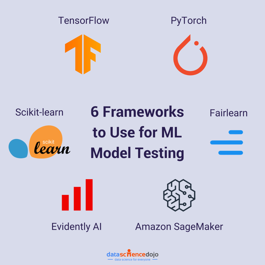
Since testing ML models is a very important task, it requires a thorough and efficient approach. Multiple frameworks in the market offer pre-built tools, enforce structured testing, provide diverse testing functionalities, and promote reproducibility.
It results in faster and more reliable testing for robust models. Here’s a list of key frameworks used for ML model testing.
TensorFlow
There are three main types of TensorFlow frameworks for testing:
TensorFlow Extended (TFX): This is designed for production pipeline testing, offering tools for data validation, model analysis, and deployment. It provides a comprehensive suite for defining, launching, and monitoring ML models in production.
TensorFlow Data Validation: Useful for testing data quality in ML pipelines.
TensorFlow Model Analysis: Used for in-depth model evaluation.
PyTorch
Known for its dynamic computation graph and ease of use, PyTorch provides model evaluation, debugging, and visualization tools. The torchvision package includes datasets and transformations for testing and validating computer vision models.
Scikit-learn
Scikit-learn is a versatile Python library that offers various algorithms and model evaluation metrics, including cross-validation and grid search for hyperparameter tuning. It is widely used for data mining, analysis, and machine learning tasks.
Fairlearn is a toolkit designed to assess and mitigate fairness and bias issues in ML models. It includes algorithms to reweight data and adjust predictions to achieve fairness, ensuring that models treat all individuals fairly and equitably.
Evidently AI
Evidently AI is an open-source Python tool that is used to analyze, monitor, and debug machine learning models in a production environment. It helps implement testing and monitoring for different model types and data types.
Amazon SageMaker Model Monitor
Amazon SageMaker is a tool that can alert developers of any deviations in model quality so that corrective actions can be taken. It supports no-code monitoring capabilities and custom analysis through coding.
These frameworks provide a comprehensive approach to testing machine learning models, ensuring they are reliable, fair, and well-performing in production environments.
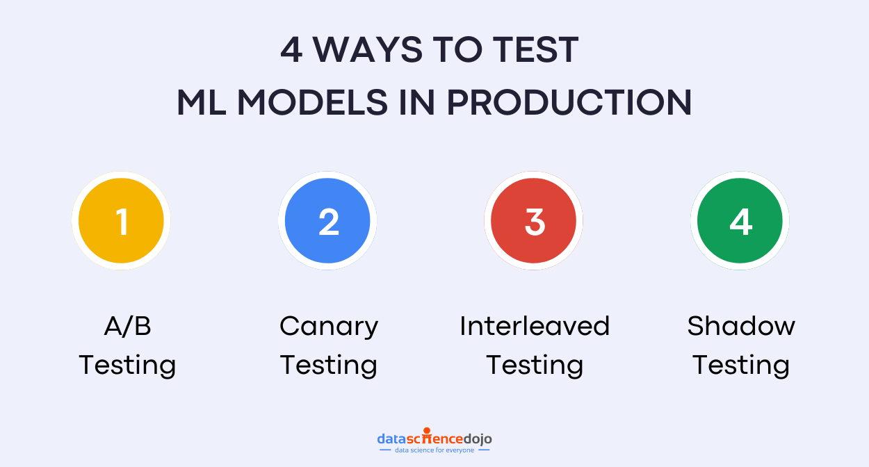
Now that we have explored the basics of ML model testing, let’s look at the 4 main testing methods for ML models in their production phase.
1. A/B Testing
Source: Medium
This is used to compare two versions of an ML model to determine which one performs better in a real-world setting. This approach is essential for validating the effectiveness of a new model before fully deploying it into production.
This helps in understanding the impact of the new model and ensuring it does not introduce unexpected issues.
It works by distributing the incoming requests non-uniformly between the two models. A smaller portion of the traffic is directed to the new model that is being tested to minimize potential risks. The performance of both models is measured and compared based on predefined metrics.
Benefits of A/B Testing
Risk Mitigation: By limiting the exposure of the candidate model, A/B testing helps in identifying any issues in the new model without affecting a large portion of users.
Performance Validation: It allows teams to validate that the new model performs at least as well as, if not better than, the legacy model in a production environment.
Data-Driven Decisions: The results from A/B testing provide concrete data to support decisions on whether to fully deploy the candidate model or make further improvements.
Thus, it is a critical testing step in ML model testing, ensuring that a new model is thoroughly vetted in a real-world environment, thereby maintaining model reliability and performance while minimizing risks associated with deploying untested models.
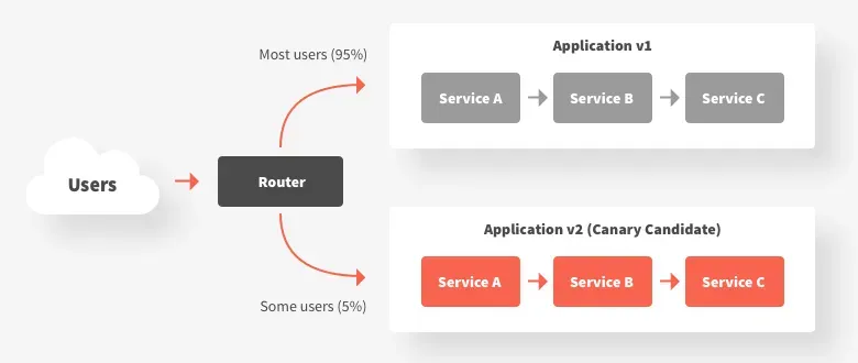
The canary testing method is used to gradually deploy a new ML model to a small subset of users in production to minimize risks and ensure that the new model performs as expected before rolling it out to a broader audience. This smaller subset of users is often referred to as the ‘canary’ group.
The main goal of this method is to limit the exposure of the new ML model initially. This incremental approach helps in identifying and mitigating any potential issues without affecting the entire user base. The performance of the ML model is monitored in the canary group.
If the model performs well in the canary group, it is gradually rolled out to a larger user base. This process continues incrementally until the new model is fully deployed to all users.
Benefits of Canary Testing
Risk Reduction: By initially limiting the exposure of the new model, canary testing reduces the risk of widespread issues affecting all users. Any problems detected can be addressed before a full-scale deployment.
Controlled Environment: This method provides a controlled environment to observe the new model’s behavior and make necessary adjustments based on real-world data.
User Impact Minimization: Users in the canary group serve as an early indicator of potential issues, allowing teams to respond quickly and minimize the impact on the broader user base.
Canary testing is an effective strategy for deploying new ML models in production. It ensures that potential issues are identified and resolved early, thereby maintaining the stability and reliability of the service while introducing new features or improvements.
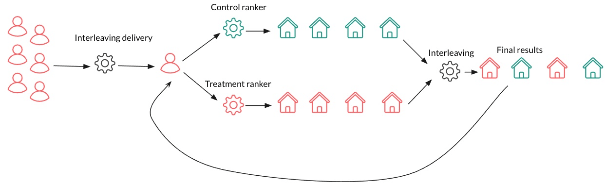
3. Interleaved Testing
A display of how interleaving works – Source: Medium
It is used to evaluate multiple ML models by mixing their outputs in real-time within the same user interface or service. This type of testing is particularly useful when you want to compare the performance of different models without exposing users to only one model at a time.
Users interact with the integrated output without knowing which model generated which part of the response. This helps in gathering unbiased user feedback and performance metrics for both models, allowing for a direct comparison under the same conditions and identifying which model performs better in real-world scenarios.
The performance of each model is tracked based on user interactions. Metrics such as click-through rates, engagement, and conversion rates are analyzed to determine which model is more effective.
Benefits of Interleaved Testing
Direct Comparison: Interleaved testing allows for a direct, side-by-side comparison of multiple models under the same conditions, providing more accurate insights into their performance.
User Experience Consistency: Since users are exposed to outputs from both models simultaneously, the overall user experience remains consistent, reducing the risk of user dissatisfaction.
Detailed Feedback: This method provides detailed feedback on how users interact with different model outputs, helping in fine-tuning and improving model performance.
Interleaved testing is a useful testing strategy that ensures a direct comparison, providing valuable insights into model performance. It helps data scientists and engineers to make informed decisions about which model to deploy.
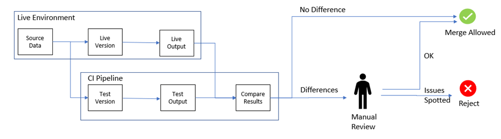
4. Shadow Testing
A glimpse of how shadow testing is implemented – Source: Medium
Shadow testing, also known as dark launching, is a technique used for real-world testing of a new ML model alongside the existing one, providing a risk-free way to gather performance data and insights.
It works by deploying both the new and old ML models in parallel. For each incoming request, the data is sent to both models simultaneously. Both models generate predictions, but only the output from the older model is served to the user. Predictions from the new ML model are logged for later analysis.
These predictions are then compared against the results of the older ML model and any available ground truth data to evaluate the performance of the new model.
Benefits of Shadow Testing
Risk-Free Evaluation: Since the candidate model’s predictions are not served to the users, any errors or issues in the new model do not affect the user experience. This makes shadow testing a safe way to test new models.
Real-World Data: Shadow testing provides insights based on real-world data and conditions, offering a more accurate assessment of the model’s performance compared to offline testing.
Benchmarking: It allows for direct comparison between the legacy and candidate models, making it easier to benchmark the new model’s performance and identify areas for improvement.
Hence, it is a robust technique for evaluating new ML models in a live production environment without impacting the user experience. It provides valuable performance insights, ensures safe testing, and helps in making informed decisions about model deployment.
How to Choose a Testing Technique for Your ML Model Testing?
Choosing the appropriate testing technique for your machine learning models in production depends on several factors, including the nature of your model, the risks associated with its deployment, and the specific requirements of your application.
Here are some key considerations and steps to help you decide on the right testing technique:
Understand the Nature and Requirements of Your Model
Different models (classification, regression, recommendation, etc.) require different testing approaches. Complex models may benefit from more rigorous testing techniques like shadow testing or interleaved testing. Hence, you must understand the nature of your model and its complexity.
Moreover, it is crucial to assess the potential impact of model errors. High-stakes applications, such as financial services or healthcare, may necessitate more conservative and thorough testing techniques.
Evaluate Common Testing Techniques
Review and evaluate the pros and cons of the testing techniques, like the 4 methods discussed earlier in the blog. A thorough understanding of the techniques can make your decision easier and more informed.
While you have multiple options available, the state of your infrastructure and available resources are strong parameters for your final decision. Ensure that your production environment can support the chosen testing technique. For example, shadow testing requires infrastructure capable of parallel processing.
You must also evaluate the available resources, including computational power, storage, and monitoring tools. Techniques like shadow testing and interleaved testing can be resource-intensive. Hence, you must consider both factors when choosing a testing technique for your ML model.
Consider Ethical and Regulatory Constraints
Data privacy and digital ethics are important parameters for modern-day businesses and users. Hence, you must ensure compliance with data privacy regulations such as GDPR or CCPA, especially when handling sensitive data.
You must choose techniques that allow for the mitigation of model bias, ensuring fairness in predictions.
Monitor and Iterate
Testing ML models in production is a continuous process. You must continuously track your model performance, data drift, and prediction accuracy over time. This must link to an iterative model improvement process. You can establish a feedback loop to retrain and update the model based on the gathered performance data.
Hence, you must carefully select the model technique for your ML model. You can consider techniques like A/B testing for direct performance comparison, canary testing for gradual rollout, interleaved testing for simultaneous output assessment, and shadow testing for risk-free evaluation.
To Sum it Up…
ML model testing when in production is a critical step. You must ensure your model’s reliability, performance, and safety in real-world scenarios. You can do that by evaluating the model’s performance in a live environment, identifying potential issues, and finding ways to resolve them.
We have explored 4 different methods to test ML models where way offers unique benefits and is suited to different scenarios and business needs. By carefully selecting the appropriate technique, you can ensure your ML models perform as expected, maintain user satisfaction, and uphold high standards of reliability and safety.
If you are interested in learning how to build ML models from scratch, here’s a video for a more engaging learning experience:
Artificial Intelligence is reshaping industries around the world, revolutionizing how businesses operate and deliver services. From healthcare where AI assists in diagnosis and treatment plans, to finance where it is used to predict market trends and manage risks, the influence of AI is pervasive and growing.
As AI technologies evolve, they create new job roles and demand new skills, particularly in the field of AI engineering. AI engineering is more than just a buzzword; it’s becoming an essential part of the modern job market. Companies are increasingly seeking professionals who can not only develop AI solutions but also ensure these solutions are practical, sustainable, and aligned with business goals.
What is AI Engineering?
AI engineering is the discipline that combines the principles of data science, software engineering, and machine learning to build and manage robust AI systems. It involves not just the creation of AI models but also their integration, scaling, and management within an organization’s existing infrastructure.
The role of an AI engineer is multifaceted. They work at the intersection of various technical domains, requiring a blend of skills to handle data processing, algorithm development, system design, and implementation.
Understand how AI as a Service (AIaaS) will transform the Industry.
This interdisciplinary nature of AI engineering makes it a critical field for businesses looking to leverage AI to enhance their operations and competitive edge.
Latest Advancements in AI Affecting Engineering
Artificial Intelligence continues to advance at a rapid pace, bringing transformative changes to the field of engineering. These advancements are not just theoretical; they have practical applications that are reshaping how engineers solve problems and design solutions.
Machine Learning Algorithms
Recent improvements in machine learning algorithms have significantly enhanced their efficiency and accuracy. Engineers now use these algorithms to predict outcomes, optimize processes, and make data-driven decisions faster than ever before.
For example, predictive maintenance in manufacturing uses machine learning to anticipate equipment failures before they occur, reducing downtime and saving costs.
Deep learning, a subset of machine learning, uses structures called neural networks which are inspired by the human brain. These networks are particularly good at recognizing patterns, which is crucial in fields like civil engineering where pattern recognition can help in assessing structural damage from images automatically.
Advances in neural networks have led to better model training techniques and improved performance, especially in complex environments with unstructured data. In software engineering, neural networks are used to improve code generation, bug detection, and even automate routine programming tasks.
Robotics combined with AI has led to the creation of more autonomous, flexible, and capable robots. In industrial engineering, robots equipped with AI can perform a variety of tasks from assembly to more complex functions like navigating unpredictable warehouse environments.
Automation
AI-driven automation technologies are now more sophisticated and accessible, enabling engineers to focus on innovation rather than routine tasks. Automation in AI has seen significant use in areas such as automotive engineering, where it helps in designing more efficient and safer vehicles through simulations and real-time testing data.
These advancements in AI are not only making engineering more efficient but also more innovative, as they provide new tools and methods for addressing engineering challenges. The ongoing evolution of AI technologies promises even greater impacts in the future, making it an exciting time for professionals in the field.
Importance of AI Engineering Skills in Today’s World
As Artificial Intelligence integrates deeper into various industries, the demand for skilled AI engineers has surged, underscoring the critical role these professionals play in modern economies.
Impact Across Industries
Healthcare
In the healthcare industry, AI engineering is revolutionizing patient care by improving diagnostic accuracy, personalizing treatment plans, and managing healthcare records more efficiently. AI tools help predict patient outcomes, support remote monitoring, and even assist in complex surgical procedures, enhancing both the speed and quality of healthcare services.
In finance, AI engineers develop algorithms that detect fraudulent activities, automate trading systems, and provide personalized financial advice to customers. These advancements not only secure financial transactions but also democratize financial advice, making it more accessible to the public.
Automotive
The automotive sector benefits from AI engineering through the development of autonomous vehicles and advanced safety features. These technologies reduce human error on the roads and aim to make driving safer and more efficient.
Economic and Social Benefits
Increased Efficiency
AI engineering streamlines operations across various sectors, reducing costs and saving time. For instance, AI can optimize supply chains in manufacturing or improve energy efficiency in urban planning, leading to more sustainable practices and lower operational costs.
As AI technologies evolve, they create new job roles in the tech industry and beyond. AI engineers are needed not just for developing AI systems but also for ensuring these systems are ethical, practical, and tailored to specific industry needs.
Innovation in Traditional Fields
AI engineering injects a new level of innovation into traditional fields like agriculture or construction. For example, AI-driven agricultural tools can analyze soil conditions and weather patterns to inform better crop management decisions, while AI in construction can lead to smarter building techniques that are environmentally friendly and cost-effective.
The proliferation of AI technology highlights the growing importance of AI engineering skills in today’s world. By equipping the workforce with these skills, industries can not only enhance their operational capacities but also drive significant social and economic advancements.
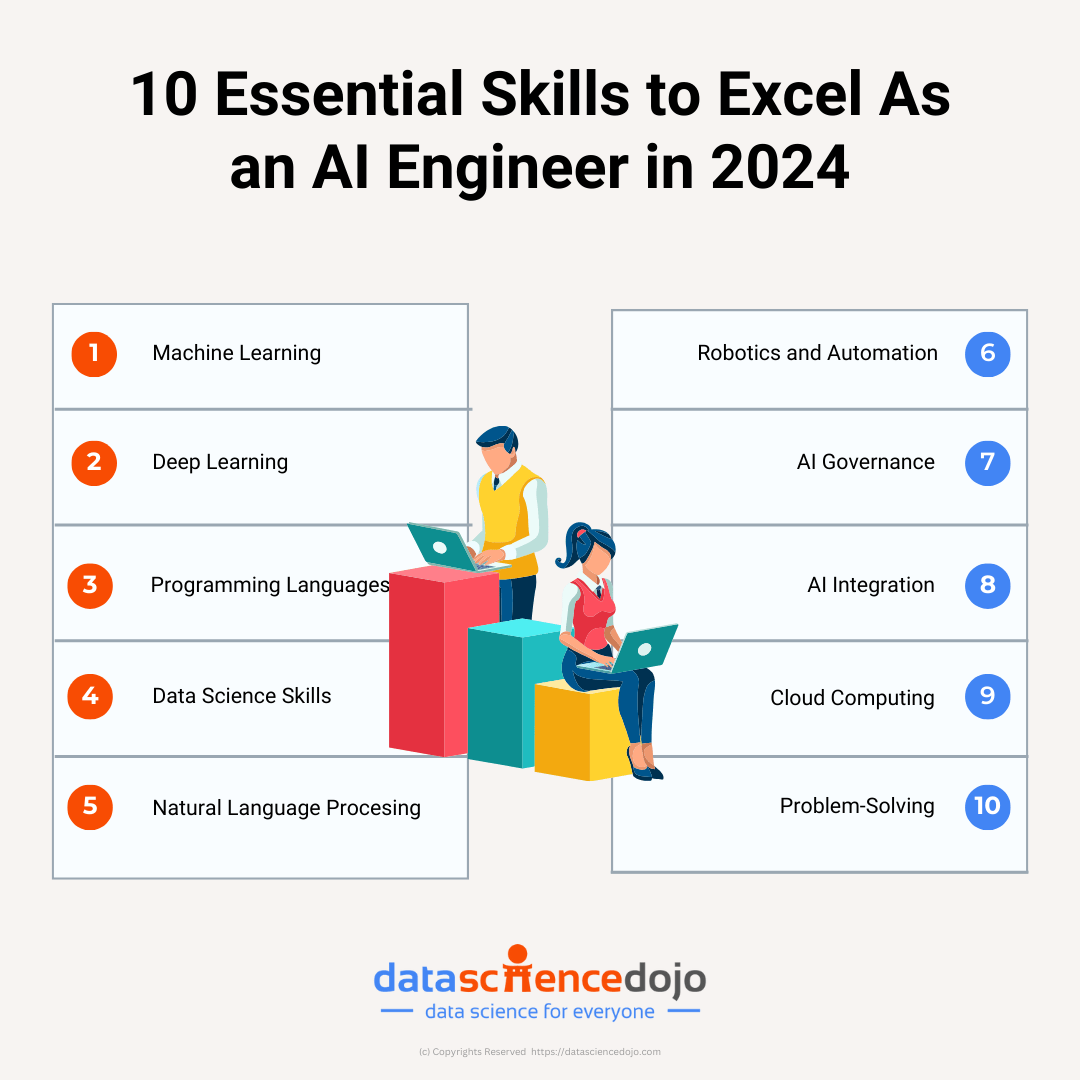
10 Must-Have AI Skills to Help You Excel
1. Machine Learning and Algorithms
Machine learning algorithms are crucial tools for AI engineers, forming the backbone of many artificial intelligence systems. These algorithms enable computers to learn from data, identify patterns, and make decisions with minimal human intervention and are divided into supervised, unsupervised, and reinforcement learning.
For AI engineers, proficiency in these algorithms is vital as it allows for the automation of decision-making processes across diverse industries such as healthcare, finance, and automotive. Additionally, understanding how to select, implement, and optimize these algorithms directly impacts the performance and efficiency of AI models.
AI engineers must be adept in various tasks such as algorithm selection based on the task and data type, data preprocessing, model training and evaluation, hyperparameter tuning, and the deployment and ongoing maintenance of models in production environments.
2. Deep Learning
Deep learning is a subset of machine learning based on artificial neural networks, where the model learns to perform tasks directly from text, images, or sounds. Deep learning is important for AI engineers because it is the key technology behind many advanced AI applications, such as natural language processing, computer vision, and audio recognition.
These applications are crucial in developing systems that mimic human cognition or augment capabilities across various sectors, including healthcare for diagnostic systems, automotive for self-driving cars, and entertainment for personalized content recommendations.
AI engineers working with deep learning need to understand the architecture of neural networks, including convolutional and recurrent neural networks, and how to train these models effectively using large datasets.
They also need to be proficient in using frameworks like TensorFlow or PyTorch, which facilitate the design and training of neural networks. Furthermore, understanding regularization techniques to prevent overfitting, optimizing algorithms to speed up training, and deploying trained models efficiently in production are essential skills for AI engineers in this domain.
3. Programming Languages
Programming languages are fundamental tools for AI engineers, enabling them to build and implement artificial intelligence models and systems. These languages provide the syntax and structure that engineers use to write algorithms, process data, and interface with hardware and software environments.
Python
Python is perhaps the most critical programming language for AI due to its simplicity and readability, coupled with a robust ecosystem of libraries like TensorFlow, PyTorch, and Scikit-learn, which are essential for machine learning and deep learning. Python’s versatility allows AI engineers to develop prototypes quickly and scale them with ease.
R is another important language, particularly valued in statistics and data analysis, making it useful for AI applications that require intensive data processing. R provides excellent packages for data visualization, statistical testing, and modeling that are integral for analyzing complex datasets in AI.
Java
Java offers the benefits of high performance, portability, and easy management of large systems, which is crucial for building scalable AI applications. Java is also widely used in big data technologies, supported by powerful Java-based tools like Apache Hadoop and Spark, which are essential for data processing in AI.
C++
C++ is essential for AI engineering due to its efficiency and control over system resources. It is particularly important in developing AI software that requires real-time execution, such as robotics or games. C++ allows for higher control over hardware and graphical processes, making it ideal for applications where latency is a critical factor.
AI engineers should have a strong grasp of these languages to effectively work on a variety of AI projects.
4. Data Science Skills
Data science skills are pivotal for AI engineers because they provide the foundation for developing, tuning, and deploying intelligent systems that can extract meaningful insights from raw data.
These skills encompass a broad range of capabilities from statistical analysis to data manipulation and interpretation, which are critical in the lifecycle of AI model development.
AI engineers need a solid grounding in statistics and probability to understand and apply various algorithms correctly. These principles help in assessing model assumptions, validity, and tuning parameters, which are crucial for making predictions and decisions based on data.
Data Manipulation and Cleaning
Before even beginning to design algorithms, AI engineers must know how to preprocess data. This includes handling missing values, outlier detection, and normalization. Clean and well-prepared data are essential for building accurate and effective models, as the quality of data directly impacts the outcome of predictive models.
Big Data Technologies
With the growth of data-driven technologies, AI engineers must be proficient in big data platforms like Hadoop, Spark, and NoSQL databases. These technologies help manage large volumes of data beyond what is manageable with traditional databases and are essential for tasks that require processing large datasets efficiently.
Machine Learning and Predictive Modeling
Data science is not just about analyzing data but also about making predictions. Understanding machine learning techniques—from linear regression to complex deep learning networks—is essential. AI engineers must be able to apply these techniques to create predictive models and fine-tune them according to specific data and business requirements.
The ability to visualize data and model outcomes is crucial for communicating findings effectively to stakeholders. Tools like Matplotlib, Seaborn, or Tableau help in creating understandable and visually appealing representations of complex data sets and results.
In sum, data science skills enable AI engineers to derive actionable insights from data, which is the cornerstone of artificial intelligence applications.
5. Natural Language Processing (NLP)
NLP involves programming computers to process and analyze large amounts of natural language data. This technology enables machines to understand and interpret human language, making it possible for them to perform tasks like translating text, responding to voice commands, and generating human-like text.
For AI engineers, NLP is essential in creating systems that can interact naturally with users, extracting information from textual data, and providing services like chatbots, customer service automation, and sentiment analysis. Proficiency in NLP allows engineers to bridge the communication gap between humans and machines, enhancing user experience and accessibility.
This field focuses on designing and programming robots that can perform tasks autonomously. Automation in AI involves the application of algorithms that allow machines to perform repetitive tasks without human intervention.
AI engineers involved in robotics and automation can revolutionize industries like manufacturing, logistics, and even healthcare, by improving efficiency, precision, and safety. Knowledge of robotics algorithms, sensor integration, and real-time decision-making is crucial for developing systems that can operate in dynamic and sometimes unpredictable environments.
Know more about 10 AI startups revolutionizing healthcare
7. Ethics and AI Governance
Ethics and AI governance encompass understanding the moral implications of AI, ensuring technologies are used responsibly, and adhering to regulatory and ethical standards. As AI becomes more prevalent, AI engineers must ensure that the systems they build are fair and transparent, and do not infringe on privacy or human rights.
This includes deploying unbiased algorithms and protecting data privacy. Understanding ethics and governance is critical not only for building trust with users but also for complying with increasing global regulations regarding AI.
8. AI Integration
AI integration involves embedding AI capabilities into existing systems and workflows without disrupting the underlying processes.
For AI engineers, the ability to integrate AI smoothly means they can enhance the functionality of existing systems, bringing about significant improvements in performance without the need for extensive infrastructure changes. This skill is essential for ensuring that AI solutions deliver practical benefits and are adopted widely across industries.
9. Cloud and Distributed Computing
This involves using cloud platforms and distributed systems to deploy, manage, and scale AI applications. The technology allows for the handling of vast amounts of data and computing tasks that are distributed across multiple locations.
AI engineers must be familiar with cloud and distributed computing to leverage the computational power and storage capabilities necessary for large-scale AI tasks. Skills in cloud platforms like AWS, Azure, and Google Cloud are crucial for deploying scalable and accessible AI solutions. These platforms also facilitate collaboration, model training, and deployment, making them indispensable in the modern AI landscape.
These skills collectively equip AI engineers to not only develop innovative solutions but also ensure these solutions are ethically sound, effectively integrated, and capable of operating at scale, thereby meeting the broad and evolving demands of the industry.
10. Problem-solving and Creative Thinking
Problem-solving and creative thinking in the context of AI engineering involve the ability to approach complex challenges with innovative solutions and a flexible mindset. This skill set is about finding efficient, effective, and sometimes unconventional ways to address technical hurdles, develop new algorithms, and adapt existing technologies to novel applications.
For AI engineers, problem-solving and creative thinking are indispensable because they operate at the forefront of technology where standard solutions often do not exist. The ability to think creatively enables engineers to devise unique models that can overcome the limitations of existing AI systems or explore new areas of AI applications.
Additionally, problem-solving skills are crucial when algorithms fail to perform as expected or when integrating AI into complex systems, requiring a deep understanding of both the technology and the problem domain.
This combination of creativity and problem-solving drives innovation in AI, pushing the boundaries of what machines can achieve and opening up new possibilities for technological advancement and application.
Empowering Your AI Engineering Career
In conclusion, mastering the skills outlined—from machine learning algorithms and programming languages to ethics and cloud computing—is crucial for any aspiring AI engineer.
These competencies will not only enhance your ability to develop innovative AI solutions but also ensure you are prepared to tackle the ethical and practical challenges of integrating AI into various industries. Embrace these skills to stay competitive and influential in the ever-evolving field of artificial intelligence.
Feature Engineering is a process of using domain knowledge to extract and transform features from raw data. These features can be used to improve the performance of Machine Learning Algorithms.
Feature Engineering encompasses a diverse array of techniques, including Feature Transformation, Feature Construction, Feature Selection, Feature Scaling, and Feature Extraction, each playing a crucial role in refining and optimizing the representation of data for machine learning tasks.
In this blog, we will discuss one of the feature transformation techniques called feature scaling with examples and see how it will be the game changer for our machine learning model accuracy.
In the world of data science and machine learning, feature transformation plays a crucial role in achieving accurate and reliable results. By manipulating the input features of a dataset, we can enhance their quality, extract meaningful information, and improve the performance of predictive models. Python, with its extensive libraries and tools, offers a streamlined and efficient process for simplifying feature scaling.
What is Feature Scaling?
Feature scaling is a crucial step in the feature transformation process that ensures all features are on a similar scale. It is the process that normalizes the range of input columns and makes it useful for further visualization and machine learning model training. The figure below shows a quick representation of feature scaling techniques that we will discuss in this blog.
A visual representation of feature scaling techniques – Source: someka.net
Why Feature Scaling is Important?
Feature scaling is important because of several factors:
It improves the machine learning model’s accuracy
It enhances the interpretability of data by transforming features on a common scale, without scaling, it is difficult to make comparisons of two features because of scale difference
It speeds up the convergence in optimization algorithms like gradient descent algorithms
It reduces the computational resources required for training the model
For better accuracy, it is essential for the algorithms that rely on distance measures, such as K-nearest neighbors (KNN) and Support Vector Machines (SVM), to be sensitive to feature scales
Now let’s dive into some important methods of feature scaling and see how they impact data understanding and machine learning model performance.
A feature scaling technique is often applied as part of data preparation for machine learning. The goal of normalization is to change the value of numeric columns in the dataset to use a common scale, without distorting differences in the range of values or losing any information.
Min-Max Scaler
The most commonly used normalization technique is min-max scaling, which transforms the features to a specific range, typically between 0 and 1. Scikit-learn has a built-in class available named MinMaxScaler that we can use directly for normalization. It involves subtracting the minimum value and dividing by the range of the feature using this formula.
Where,
Xi is the value we want to normalize.
Xmaxis the maximum value of the feature.
Xminis the minimum value of the feature.
In this transformation, the mean and standard deviation of the feature may behave differently. Our main focus in this normalization is on the minimum and maximum values. Outliers may disrupt our data pattern, so taking care of them is necessary.
Let’s take an example of a wine dataset that contains various ingredients of wine as features. We take two input features: the quantity of alcohol and malic acid and create a scatter plot as shown below.
Scatter plot from the wine dataset
When we create a scatter plot between alcohol and malic acid quantities, we can see that min-max scaling simply compresses our dataset into the range of zero to one, while keeping the distribution unchanged.
Standardization
Standardization is a feature scaling technique in which values of features are centered around the mean with unit variance. It is also called Z-Score Normalization. It subtracts the mean value of the feature and divides by the standard deviation (σ) of the feature using the formula:
Here we leverage a dataset on social network ads to gain a practical understanding of the concept. This dataset includes four input features: User ID, Gender, Age, and Salary. Based on this information, it determines whether the user made a purchase or not (where zero indicates not purchased, and one indicates purchased).
The first five rows of the dataset appear as follows:
Dataset for the standardization example
In this example, we extract only two input features (Age and Salary) and use them to determine whether the output indicates a purchase or not as shown below.
Standard Scaler
We use Standard-Scaler from the Scikit-learn preprocessing module to standardize the input features for this feature scaling technique. The following code demonstrates this as shown.
We can see how our features look before and after standardization below.
Although it appears that the distribution changes after scaling,let’s visualize both distributions through a scatter plot.
Visual representation of the impact of scaling on data
So, when we visualize these distributions through plots, we observe that they remain the same as before. This indicates that scaling doesn’t alter the distribution; it simply centers it around the origin.
Now let’s see what happens when we create a density plot between Age and Estimated Salary with and without scaled features as shown below.
Graphical representation of data standardization
In the first plot, we can observe that we are unable to visualize the plot effectively and are not able to draw any conclusions or insights between age and estimated salary due to scale differences. However, in the second plot, we can visualize it and discern how age and estimated salary relate to each other.
This illustrates how scaling assists us by placing the features on similar scales. Note that this technique does not have any impact on outliers. So, if an outlier is present in the dataset, it remains as it is even after standardization. Therefore, we need to address outliers separately.
Model’s Performance Comparison
Now we use the logistic regression technique to predict whether a person will make a purchase after seeing an advertisement and observe how the model behaves with scaled features compared to without scaled features.
Here, we can observe a drastic improvement in our model accuracy when we apply the same algorithm to standardized features. Initially, our model accuracy is around 65.8%, and after standardization, it improves to 86.7%
When Does It Matter?
Note that standardization does not always improve your model accuracy; its effectiveness depends on your dataset and the algorithms you are using. However, it can be very effective when you are working with multivariate analysis and similar methods, such as Principal Component Analysis (PCA), Support Vector Machine (SVM), K-means, Gradient Descent, Artificial Neural Networks (ANN), and K-nearest neighbors (KNN).
However, when you are working with algorithms like decision trees, random forest, Gradient Boosting (G-Boost), and (X-Boost), standardization may not have any impact on improving your model accuracy as these algorithms work on different principles and are not affected by differences in feature scales
To Sum It Up
We have covered standardization and normalization as two methods of feature scaling, including important techniques like Standard Scaler and Min-Max Scaler. These methods play a crucial role in preparing data for machine learning models, ensuring features are on a consistent scale. By standardizing or normalizing data, we enhance model performance and interpretability, paving the way for more accurate predictions and insights.
Imagine a world where your business could make smarter decisions, predict customer behavior with astonishing accuracy, and automate tasks that used to take hours. That world is within reach through machine learning (ML).
In this machine learning guide, we’ll take you through the end-to-end ML process in business, offering examples and insights to help you understand and harness its transformative power. Whether you’re just starting with ML or want to dive deeper, this guide will equip you with the knowledge to succeed.
Let’s simplify the machine learning process into clear, actionable steps. No jargon—just what you need to know to build, deploy, and maintain models that work.
1.Nail Down the Problem
When it comes to machine learning, success starts long before you write a single line of code—it begins with defining the problem clearly.
Begin by asking yourself: “What is the specific problem I’m solving?” This might sound obvious, but the clarity of your initial problem statement can make or break your project. Instead of a vague goal like “improve sales,” refine your objective to something actionable and measurable. For example:
Clear Objective: “Predict which customers will buy Product X in the next month using their browsing history.”
This level of specificity helps ensure that your efforts are laser-focused and aligned with your business needs.
Real-World Examples
To see this in action, consider how industry leaders have tackled their challenges:
Netflix: Their challenge wasn’t just about keeping users entertained—it was about engaging them through personalized recommendation engines. Netflix’s ML models analyze viewing habits to suggest content that keeps users coming back for more.
PayPal: For PayPal, the problem was ensuring security without compromising user experience. They developed real-time transaction analysis systems that detect and prevent fraud almost instantaneously, all while minimizing inconvenience for genuine users.
Both examples underscore the importance of pinpointing the problem. A well-defined challenge paves the way for a tailored Machine Learning solution that directly addresses key business objectives.
Pro Tips for Getting Started
Test If ML Is Necessary: Sometimes, traditional analytics like trend reports or descriptive statistics might solve the problem just as well. Evaluate whether the complexity of Machine learning is warranted before proceeding.
Set Success Metrics Early:
Accuracy: Determine what level of accuracy is acceptable for your application. For instance, is 85% accuracy sufficient, or do you need more precision?
Speed: Consider the operational requirements. Does the model need to make decisions in milliseconds (such as for fraud detection), or can it operate on a slower timescale (like inventory restocking)?
By asking these questions upfront, you ensure that your project is grounded in realistic expectations and measurable outcomes.
2.Data: Gather, Clean, Repeat
Data is the lifeblood of any machine learning project. No matter how sophisticated your algorithm is, its performance is directly tied to the quality and relevance of the data it learns from. Let’s break down how to gather, clean, and prepare your data for success.
What to Collect
The first step is to identify and collect the right data. Your goal is to pinpoint datasets that directly address your problem.
Here are two industry examples to illustrate this:
Walmart’s Stock Optimization: Walmart integrates multiple data sources—sales records, weather forecasts, and shipping times—to accurately predict stock needs. This multifaceted approach ensures that inventory is managed proactively, reducing both overstock and stockouts.
GE’s Predictive Maintenance: GE monitors sensor data from jet engines to predict potential mechanical failures. By collecting real-time operational data, they can flag issues before they escalate into costly failures, ensuring safety and efficiency.
In both cases, the data is specifically chosen because it has a clear, actionable relationship with the business objective. Determine the signals that matter most to your problem, and focus your data collection efforts there.
Cleaning Hacks
Raw data rarely comes perfectly packaged. Here’s how to tackle the common pitfalls:
Fix Missing Values: Data gaps are inevitable. You can fill missing values using simple imputation methods like the mean or median of the column. Alternatively, you might opt for algorithms like XGBoost, which can handle missing data gracefully without prior imputation.
Eliminate Outliers: Outliers can distort your model’s understanding of the data. For instance, encountering a record like “10 million purchase” in a dataset of 100 orders likely indicates a typo. Such anomalies should be identified and either corrected or removed to maintain data integrity.
Cleaning your data isn’t a one-time step—it’s an iterative process. As you refine your dataset, continue to clean and adjust until your data is as accurate and consistent as possible.
Formatting for Success
After cleaning, you need to format your data so that machine learning algorithms can make sense of it:
Convert Categorical Data: Many datasets contain categorical variables (e.g., “red,” “blue,” “green”). Algorithms require numerical input, so you’ll need to convert these using techniques like one-hot encoding, which transforms each category into a binary column.
Normalize Scales: Features in your data can vary drastically in scale. For example, “income” might range from 0 to 100,000, whereas “age” ranges from 0 to 100. Normalizing these features ensures that no single feature dominates the learning process, leading to fairer and more balanced results.
Proper formatting not only prepares the data for modeling but also enhances the performance and interpretability of your machine learning model.
Toolbox
Choosing the right tools for data manipulation is crucial:
Python’s Pandas: For small to medium-sized datasets, Pandas is an invaluable library. It offers robust data manipulation capabilities, from cleaning and transforming data to performing exploratory analysis with ease.
Apache Spark: When dealing with large-scale datasets or requiring distributed computing, Apache Spark becomes indispensable. Its ability to handle big data efficiently makes it ideal for complex data wrangling tasks, ensuring scalability and speed.
Choosing the right model is a critical step in your machine learning journey. The model you select should align perfectly with your problem type and the nature of your data. Here’s how to match your problem with the appropriate algorithm and set yourself up for training success.
Match Your Problem to the Algorithm
Supervised Learning (When You Have Labeled Data)
Supervised learning is your go-to when you have clear, labeled examples in your dataset. This approach lets your model learn a mapping from inputs to outputs.
Predicting Numbers: For tasks like estimating house prices or forecasting sales, linear regression is often the best starting point. It’s designed to predict continuous values by finding a relationship between independent variables and a target number.
Classifying Categories: When your objective is to sort data into categories (think spam vs. not spam emails), decision trees can be a powerful tool. They split data into branches to help make decisions based on feature values, providing clear, interpretable results.
Unsupervised Learning (When Labels Are Absent)
Sometimes, your data won’t come with labels, and your goal is to uncover hidden structures or patterns. This is where unsupervised learning shines.
Grouping Users: To segment customers or users into meaningful clusters, K-means clustering is highly effective. For example, Spotify might use clustering techniques to segment users based on listening habits, enabling personalized playlist recommendations without any pre-defined labels.
Training Secrets
Once you’ve matched your problem with an algorithm, these training tips will help ensure your model performs well:
Split Your Data: Avoid overfitting by dividing your dataset into a training set (about 80%) and a validation set (around 20%). This split lets you train your model on one portion of the data and then validate its performance on unseen data, ensuring it generalizes well.
Start Simple: Don’t jump straight into complex models. A basic model, such as logistic regression for classification tasks, can often outperform a more complex neural network if the latter isn’t well-tuned. Begin with simplicity, and only increase complexity as needed based on your model’s performance and the intricacies of your data.
Testing your machine learning model in a controlled environment is only the beginning. A model that works perfectly in the lab might stumble when faced with real-world data. That’s why a rigorous cycle of testing, tweaking, and repeating is essential to refine your model until it meets your performance benchmarks in practical settings.
Metrics That Matter
Before you dive into adjustments, you need to know how well your model is performing. Here are a few key metrics to track:
Accuracy: This tells you the percentage of correct predictions your model makes. While it’s a useful starting point, accuracy alone can be misleading, especially with imbalanced datasets.
Precision: Precision measures the percentage of positive identifications (for example, fraud alerts) that are actually correct. In a fraud detection scenario, high precision means that most flagged transactions are genuinely fraudulent, minimizing false alarms.
Recall: Recall is the percentage of total actual positive cases (like actual fraud cases) that your model successfully identifies. A model with high recall catches more instances of fraud, though it may also increase false positives if not balanced properly.
These metrics provide a multi-faceted view of your model’s performance, ensuring you don’t overlook important aspects like the cost of false positives or negatives.
The Fix-It Playbook
Once you’ve established your performance metrics, it’s time to refine your model with some targeted tweaks:
Tweak Hyperparameters: Every algorithm comes with its own set of hyperparameters that control how fast a neural network learns, the depth of decision trees, or the regularization strength in regression models. Experimenting with these settings can significantly improve model performance. For example, adjusting the learning rate in a neural network might prevent it from overshooting the optimal solution.
Address Imbalanced Data: Many real-world datasets are imbalanced. In a fraud detection scenario, you might find that 99% of transactions are legitimate while only 1% are fraudulent. This imbalance can cause your model to lean towards predicting the majority class. One effective strategy is to oversample the rare class (fraud cases) or use techniques like Synthetic Minority Over-sampling Technique (SMOTE) to create a more balanced dataset.
Iterative Testing: Once you’ve made your adjustments, it’s crucial to revalidate your model. Does it still perform well on your validation set? Are there any new errors or biases that have emerged? Continuous testing and validation help ensure your tweaks lead to real improvements rather than unintended consequences.
Red Flag: Revisit Your Data
If your model fails to meet the expected performance during validation, consider revisiting your data:
Hidden Patterns: It might be that important signals or patterns in your data are being missed. Perhaps there’s a subtle correlation or a feature interaction that wasn’t captured during initial data preparation. Going back to your data, exploring it further, and even gathering more relevant data can sometimes be the missing piece of the puzzle.
Data Quality Issues: Re-examine your data cleaning process. Incomplete, noisy, or biased data can lead your model astray. Make sure your data preprocessing steps—like handling missing values and eliminating outliers—are robust enough to support your model’s learning process.
When it comes to deploying your machine learning model, remember: Launch Smart, Not Fast. This is where theory meets reality, and even the most promising model must prove its worth under real-world conditions. Before you hit the deploy button, consider the following aspects to ensure a smooth transition from development to production.
Ask the Right Questions
Before deployment, it’s crucial to understand how your model will operate in its new environment:
Real-Time vs. Batch Predictions: Ask yourself, “Will predictions happen in real-time or in batches?” For example, a fraud detection system demands instant, real-time responses, whereas a model generating nightly sales forecasts can work on a batch schedule. The decision here affects both the design and the infrastructure you’ll need.
Data Ingestion: Determine how your model will receive new data once it’s deployed. Will it integrate via APIs, or will it rely on direct database feeds? The method of data integration can influence both the model’s performance and its reliability in production.
Tools to Try
Leveraging the right tools can streamline your deployment process and help you scale efficiently:
Cloud Platforms: Consider using cloud services like AWS SageMaker or Google AI Platform. These platforms not only simplify deployment but also offer scalability and management features that ensure your model can handle increasing loads as your user base grows.
Edge Devices: If your model needs to run on mobile phones, IoT sensors, or other edge devices, frameworks like TensorFlow Lite are invaluable. They enable you to deploy lightweight models that can operate efficiently on devices with limited computational power, ensuring quick responses and reducing latency.
Once your machine learning model is live, the journey is far from over. The real world is in constant flux, and your model must evolve along with it. Monitoring your model is not a one-time event—it’s a continuous process that ensures your model remains accurate, relevant, and effective as data changes over time.
The Challenge: Model Degradation
No matter how well you build your model, it can degrade as the underlying data evolves. Two key phenomena to watch out for are:
Data Drift: Over time, the statistical properties of your input data can change. For example, customer habits might shift dramatically—think of the surge in online shopping post-pandemic. When your model is trained on outdated data, its predictions may no longer reflect current trends.
Concept Drift: This occurs when the relationship between input features and the target output shifts. A classic case is inflation altering spending patterns; even if the data seems consistent, the underlying dynamics can change, causing your model’s accuracy to slip.
Your Survival Kit for Continuous Monitoring
To ensure your model stays on track, it’s crucial to implement a robust monitoring and updating strategy. Here’s how to keep your model in peak condition:
Regular Retraining: Schedule regular intervals for retraining your model—monthly might work for many applications, but industries like finance, where market conditions shift rapidly, may require weekly updates. Regular retraining helps incorporate the latest data and adjust to any emerging trends.
A/B Testing: Don’t simply replace your old model with a new one without evidence of improvement. Use A/B testing to compare the performance of the new model against the old version. This approach provides clear insights into whether the new model is genuinely better or if further adjustments are needed.
Performance Dashboards: Set up real-time dashboards that track key performance metrics such as accuracy, precision, recall, and other domain-specific measures. These dashboards serve as an early warning system, alerting you when performance starts to degrade.
Automated Alerts: Implement automated alerts to notify you when your model’s performance dips below predefined thresholds. Early detection allows you to quickly investigate and address issues before they impact your operations.
Leading Businesses Using Machine Learning Applications
Airbnb:
Airbnb stands out as a prime case study in any machine learning guide, showcasing how advanced algorithms can revolutionize business operations and elevate customer experiences. By integrating cutting-edge ML applications, Airbnb optimizes efficiency while delivering hyper-personalized services for guests and hosts.
Here’s how they leverage machine learning—a blueprint that doubles as a practical machine learning guide for businesses:
Predictive Search
Airbnb’s predictive search is designed to make finding the perfect stay as intuitive as possible. Here’s how it works:
Tailored Recommendations: By analyzing guest preferences—such as past bookings, search history, and favored amenities—along with detailed property features like location, design, and reviews, Airbnb’s system intelligently ranks listings that are most likely to meet a guest’s expectations.
Enhanced User Experience: This targeted approach reduces the time users spend sifting through irrelevant options. Instead, they see listings that best match their unique tastes and needs, leading to a smoother booking process and higher conversion rates.
Image Classification
In the hospitality industry, a picture is worth a thousand words. Airbnb leverages image classification to ensure that every listing showcases its most appealing aspects:
Automatic Photo Tagging: Advanced algorithms automatically analyze and categorize property photos. They highlight key features—like breathtaking views, cozy interiors, or modern amenities—making it easier for potential guests to assess a property at a glance.
Improved Listing Quality: By consistently presenting high-quality images that accentuate a property’s strengths, Airbnb helps hosts attract more interest and bookings. This automated process not only saves time but also maintains a uniform standard of visual appeal across the platform.
Dynamic Pricing
Pricing can make or break a booking. Airbnb’s dynamic pricing model uses machine learning to help hosts stay competitive while ensuring guests receive fair value:
Real-Time Data Analysis: The system factors in variables such as current demand, seasonal trends, local events, and historical booking data. By doing so, it suggests optimal pricing tailored to each property and market condition.
Maximized Revenue and Occupancy: For hosts, this means pricing that adapts to market fluctuations—maximizing occupancy and revenue without the guesswork. For guests, dynamic pricing can translate into competitive rates and more transparent pricing strategies.
Tinder has become a leader in the dating app industry by using machine learning to improve user experience, match accuracy, and protect against fraud. In this machine learning guide, we’ll take a closer look at how Tinder uses machine learning to enhance its platform and make the dating experience smarter and safer.
Personalized Recommendations
Tinder’s recommendation engine uses machine learning to ensure users are presented with matches that fit their preferences and behaviors:
Behavioral Analysis: Tinder analyzes user data such as swiping patterns, liked profiles, and even message interactions to understand a user’s tastes and dating preferences. This data is used to suggest potential matches who share similar interests, hobbies, or other key attributes.
Dynamic Matching: The algorithm continuously adapts to evolving user preferences, ensuring that each match suggestion is more accurate over time. This personalization enhances user engagement, as people are more likely to find compatible matches quickly.
Image Recognition
Photos play a critical role in dating app interactions, and Tinder uses image recognition to boost the relevance of its matching system:
Automatic Classification: Tinder uses machine learning algorithms to analyze and classify user-uploaded photos. This helps the app understand visual preferences—such as identifying users’ facial expressions, body language, and context (e.g., group photos or solo shots)—to present images that align with other users’ preferences.
Enhanced Match Accuracy: By considering photo content, Tinder enhances the quality of match suggestions, ensuring that visual appeal aligns with the personality and interests of both users. This also improves user confidence in the matching process by providing more relevant, visually engaging profiles.
Fraud Detection
Preventing fraudulent activity is crucial in maintaining trust on a platform like Tinder. Machine learning plays a significant role in detecting fake profiles and scams:
Profile Verification: Tinder uses advanced algorithms to analyze profile behavior and detect inconsistencies that might suggest fraudulent activity. This includes analyzing rapid, suspicious activity, such as multiple account creations or unusual swiping patterns that are characteristic of bots or fake accounts.
Fake Image Detection: Image recognition technology also helps identify potentially fake or misleading profile pictures by cross-referencing images from public databases to detect stolen or artificially altered photos.
Safety for Users: By continuously monitoring for fraudulent behavior, Tinder ensures a safer environment for users. This not only improves the overall trustworthiness of the platform but also reduces the chances of users falling victim to scams or malicious profiles.
Spotify:
Spotify has revolutionized the way people discover and enjoy music, and much of its success is driven by the power of machine learning. Here’s how Spotify uses machine learning to personalize the music experience for each user. In this machine learning guide, we’ll explore how Spotify uses machine learning to personalize the music experience for each user:
Personalized Playlists
Spotify’s recommendation engine analyzes user listening habits to create highly personalized playlists. This includes:
User Behavior Analysis: The app tracks everything from the songs you skip to the ones you repeat, and even the time of day you listen to music. This data is used to create customized playlists that fit your unique listening preferences, ensuring that every playlist feels tailor-made for you.
Tailored Artist Suggestions: Based on listening history, Spotify suggests new songs or artists that align with your taste. For instance, if you regularly listen to indie rock, you might receive new recommendations in that genre, making your music discovery seamless and more enjoyable.
Discover Weekly
Every week, Spotify generates a personalized playlist known as Discover Weekly—a unique collection of songs that users are likely to enjoy but haven’t heard before. Here’s how it works:
Collaborative Filtering: Spotify uses collaborative filtering to recommend songs based on similar listening patterns from other users. The algorithm identifies users with comparable tastes and suggests tracks that they’ve enjoyed, which the system predicts you might also like.
Constant Learning: The more you use Spotify, the better the algorithm gets at tailoring your weekly playlist. It learns from your likes, skips, and skips-to-replay patterns to refine the recommendations over time, ensuring that each week’s playlist feels fresh and aligned with your current mood and preferences.
Audio Feature Analysis
In addition to analyzing listening behavior, Spotify also uses machine learning to evaluate the audio features of songs themselves:
Analyzing Audio Features: Spotify’s algorithm looks at musical attributes such as tempo, rhythm, mood, and key to assess similarities between songs. This allows the platform to recommend tracks that sound alike, helping users discover new music that fits their preferred style, whether they want something energetic, relaxing, or melancholic.
Mood-Based Recommendations: Spotify’s machine learning models also help match users’ moods with the right music. For example, if you tend to listen to slower, melancholic songs in the evening, the system will recommend similar tracks that align with that mood.(Source)
Conclusion
Machine learning doesn’t have to be intimidating. This guide breaks down the basics into bite-sized pieces that you can build on, whether you’re just starting out or looking to polish your skills. Remember, learning ML is all about experimenting, making mistakes, and gradually improving. Keep exploring, practicing, and most importantly, have fun with it. Thanks for joining us on this journey into the world of machine learning!
In the realm of machine learning, data is the cornerstone of effective model training and performance. However, acquiring high-quality, diverse, and privacy-compliant datasets can be a daunting task. That’s where synthetic data in machine learning comes into play.
Synthetic data is generated artificially rather than sourced from real-world environments, providing a powerful solution to challenges like data scarcity, privacy concerns, and bias in machine learning models.
From boosting AI model performance to ensuring compliance with data regulations, synthetic data offers a multitude of applications across various industries. In this article, we delve into seven compelling reasons why synthetic data is indispensable and how it can propel innovation in machine learning.
To train machine learning models, you need data. However, collecting and labeling real-world data can be costly, time-consuming, and inaccurate. Synthetic data offers a solution to these challenges.
Scalability: Easily generate synthetic data for large-scale projects.
Accuracy: Synthetic data can match real data quality.
Privacy: No need to collect personal information.
Safety: Generate safe data for accident prevention.
Why do you need Synthetic Data in Machine Learning?
In the realm of machine learning, the foundation of successful models lies in high-quality, diverse, and well-balanced datasets. To achieve accuracy, models need data that mirrors real-world scenarios accurately. Some of the key features of synthetic data include:
Realistic Yet Artificial: Synthetic data mirrors real-world data distributions while being artificially created, preserving statistical properties without posing privacy risks.
Scalable and Customizable: Unlike real-world data, synthetic data can be generated in vast quantities and tailored to meet specific model requirements.
Inherently Privacy-Compliant: As synthetic data doesn’t originate from real users, it naturally aligns with data protection laws like GDPR and CCPA.
Wide Applicability Across Domains: Synthetic data is utilized in sectors like healthcare, finance, retail, and autonomous systems, making it a versatile tool across industries.
Synthetic data, which replicates the statistical properties of real data, serves as a crucial solution to address the challenges posed by data scarcity and imbalance. This article delves into the pivotal role that synthetic data plays in enhancing model performance, enabling data augmentation, and tackling issues arising from imbalanced datasets.
Improving model performance
Synthetic data serves as a powerful catalyst for improving machine learning models. It expands and enriches existing datasets by introducing artificial samples that closely mimic real-world data, making models more robust, diverse, and reliable.
How Synthetic Data Improves Machine Learning Models
Reduces Overfitting Models trained on limited real-world data often struggle with overfitting. Synthetic data introduces additional variability, preventing models from memorizing patterns and improving generalization.
Enhances Generalization By generating synthetic samples with statistical patterns similar to real-world data, models learn to recognize underlying trends rather than just specific instances. This leads to better adaptability to new, unseen data.
Improves Accuracy With a more diverse training set, models gain exposure to edge cases and rare scenarios, leading to higher accuracy and better predictions across different conditions.
Balances Imbalanced Datasets Many real-world datasets suffer from class imbalances. Synthetic data helps by creating more samples for underrepresented classes, ensuring fairer and more balanced training.
Enables Privacy-Preserving AI In cases where real-world data is sensitive or regulated (e.g., healthcare or finance), synthetic data provides a privacy-friendly alternative, allowing AI development without compromising user confidentiality.
By leveraging synthetic data, machine learning models become more efficient, scalable, and capable of handling real-world complexities with greater precision.
Data augmentation is a widely used technique in machine learning that enhances training datasets by creating diverse variations of existing samples. This helps models gain a broader understanding of the data distribution and improves their ability to generalize.
How Synthetic Data Enhances Data Augmentation
Expands Training Data Synthetic data introduces new, artificially generated samples that closely resemble real-world data, increasing dataset diversity without requiring additional real data collection.
Improves Model Robustness By generating varied versions of existing data, models learn to recognize patterns under different conditions, making them more adaptable to real-world variations.
Enhances Image Classification Performance In image classification, synthetic data can be used to create augmented images with:
Different lighting conditions
Rotations and flips
Scaling and distortions
Color transformations
Reduces Overfitting Augmenting data with synthetic variations prevents models from becoming too reliant on specific features, reducing overfitting and improving generalization.
Supports Rare Scenario Training Real-world datasets often lack rare or edge-case scenarios. Synthetic data helps fill these gaps, ensuring models are trained on a wider range of possibilities.
By integrating synthetic data into data augmentation, machine learning models become more resilient, adaptive, and capable of handling real-world complexities with greater precision.
Handling Imbalanced Datasets
Imbalanced datasets, where certain classes have significantly fewer samples than others, create challenges for machine learning models. Models trained on such datasets tend to favor the majority class, leading to biased predictions and poor performance on minority classes.
How Synthetic Data Helps Balance Datasets
Generates More Samples for Minority Classes Synthetic data can be created specifically for underrepresented classes, increasing their presence in the dataset and ensuring the model gets sufficient exposure to all classes.
Prevents Model Bias When trained on imbalanced data, models often lean towards predicting the dominant class. Synthetic data helps balance the class distribution, ensuring fairer and more accurate predictions.
Improves Model Generalization By introducing diverse synthetic samples, models learn to identify patterns in both majority and minority classes, enhancing their ability to generalize across different data points.
Enhances Classification Accuracy With a more balanced dataset, models can make more precise predictions across all classes, leading to higher overall performance and improved decision-making.
Supports Rare Event Detection In fields like fraud detection, medical diagnosis, and fault prediction, minority class instances are often the most critical. Synthetic data helps create more training examples, enabling models to better detect rare events.
By leveraging synthetic data in machine learning models become more reliable, unbiased, and effective in handling real-world scenarios where class imbalances are common.
Benefits and Considerations
Leveraging synthetic data in machine learning presents a multitude of benefits. It reduces reliance on scarce or sensitive real data, enabling researchers and practitioners to work with more extensive and diverse datasets. This, in turn, leads to improved model performance, shorter development cycles, and reduced data collection costs.
Furthermore, synthetic data can simulate rare or extreme events, allowing models to learn and respond effectively in challenging scenarios.
However, it is imperative to consider the limitations and potential pitfalls associated with the use of synthetic data. The synthetic data generated must faithfully replicate the statistical characteristics of real data to ensure models generalize effectively.
Rigorous evaluation metrics and techniques should be employed to assess the quality and utility of synthetic datasets. Ethical concerns, including privacy preservation and the inadvertent introduction of biases, demand meticulous attention when both generating and utilizing synthetic data.
Applications of Synthetic Data
Following indicates key applications of synthetic data:
Enhancing Model Training with Data Augmentation: Machine learning models thrive on diverse datasets to perform well. Synthetic data helps by expanding dataset size, reducing the risk of overfitting, and enhancing model accuracy.
Ensuring Privacy in AI Development: Real-world data often includes sensitive information. Synthetic data mitigates privacy risks by substituting real data with artificial yet statistically similar versions, ensuring compliance with regulations like GDPR and HIPAA.
Simulating Rare Scenarios and Edge Cases: Gathering real-world data on rare events, such as medical anomalies or autonomous driving challenges, is tough. Synthetic data allows AI models to learn from simulated scenarios, boosting their robustness in real-world situations.
Cutting Down Data Collection Costs: Obtaining high-quality labeled datasets is both costly and time-consuming. Synthetic data offers a cost-effective alternative, minimizing the need for extensive manual data collection and annotation.
Promoting Fairness and Reducing Bias in AI: Real-world datasets can be biased, resulting in unfair AI outcomes. Synthetic data helps balance datasets by producing diverse samples, thus enhancing fairness in machine learning models.
Advancing Cybersecurity and Fraud Detection: Synthetic datasets can train AI models to detect fraud and cybersecurity threats without risking exposure of actual confidential data, ensuring safer and privacy-compliant security training.
Speeding Up AI Research and Prototyping: Rapid experimentation is key in AI model development. Synthetic data accelerates research by supplying on-demand datasets, enabling quicker testing and validation of models.
In conclusion, synthetic data in machine learning emerges as a potent tool, addressing the challenges posed by data scarcity, diversity, and class imbalance. It unlocks the potential for heightened accuracy, robustness, and generalization in machine learning models.
Nevertheless, a meticulous evaluation process, rigorous validation, and an unwavering commitment to ethical considerations are indispensable to ensure the responsible and effective use of synthetic data in real-world applications.
Final Thoughts
Synthetic data in machine learning enhances models by addressing data scarcity, diversity, and class imbalance. It unlocks potential accuracy, robustness, and generalization. However, rigorous evaluation, validation, and ethical considerations are essential for responsible real-world use.
Whether it’s for training resilient AI models, cutting costs, or bolstering security, synthetic data is a revolutionary tool. As AI continues to advance, leveraging synthetic data will be pivotal in driving innovation and ensuring the ethical development of AI systems.
ML models have grown significantly in recent years, and businesses increasingly rely on them to automate and optimize their operations. However, managing ML models can be challenging, especially as models become more complex and require more resources to train and deploy. This has led to the emergence of MLOps as a way to standardize and streamline the ML workflow.
MLOps emphasizes the need for continuous integration and continuous deployment (CI/CD) in the ML workflow, ensuring that models are updated in real-time to reflect changes in data or ML algorithms. This infrastructure is valuable in areas where accuracy, reproducibility, and reliability are critical, such as healthcare, finance, and self-driving cars.
By implementing MLOps, organizations can ensure that their ML models are continuously updated and accurate, helping to drive innovation, reduce costs, and improve efficiency.
What is MLOps?
MLOps is a methodology combining ML and DevOps practices to streamline developing, deploying, and maintaining ML models. MLOps share several key characteristics with DevOps, including:
CI/CD: MLOps emphasizes the need for a continuous cycle of code, data, and model updates in ML workflows. This approach requires automating as much as possible to ensure consistent and reliable results.
Automation: Like DevOps, MLOps stresses the importance of automation throughout the ML lifecycle. Automating critical steps in the ML workflow, such as data processing, model training, and deployment, results in a more efficient and reliable workflow.
Collaboration and transparency: MLOps encourages a collaborative and transparent culture of shared knowledge and expertise across teams developing and deploying ML models. This helps to ensure a streamlined process, as handoff expectations will be more standardized.
Infrastructure as Code (IaC): DevOps and MLOps employ an “infrastructure as code” approach, in which infrastructure is treated as code and managed through version control systems. This approach allows teams to manage infrastructure changes more efficiently and reproducibly.
Testing and monitoring: MLOps and DevOps emphasize the importance of testing and monitoring to ensure consistent and reliable results. In MLOps, this involves testing and monitoring the accuracy and performance of ML models over time.
Flexibility and agility: DevOps and MLOps emphasize flexibility and agility in response to changing business needs and requirements. This means being able to rapidly deploy and iterate on ML models to keep up with evolving business demands.
The bottom line is that ML has a lot of variability in its behavior, given that models are essentially a black box used to generate some prediction. While DevOps and MLOps share many similarities, MLOps requires a more specialized set of tools and practices to address the unique challenges posed by data-driven and computationally intensive ML workflows.
ML workflows often require a broad range of technical skills that go beyond traditional software development, and they may involve specialized infrastructure components, such as accelerators, GPUs, and clusters, to manage the computational demands of training and deploying ML models.
Nevertheless, taking the best practices of DevOps and applying them across the ML workflow will significantly reduce project times and provide the structure ML needs to be effective in production.
Importance and benefits of MLOps in modern business
ML has revolutionized how businesses analyze data, make decisions, and optimize operations. It enables organizations to create powerful, data-driven models that reveal patterns, trends, and insights, leading to more informed decision-making and more effective automation.
However, effectively deploying and managing ML models can be challenging, which is where MLOps comes into play. MLOps is becoming increasingly important for modern businesses because it offers a range of benefits, including:
Faster development time: It allows organizations to accelerate the development life-cycle of ML models, reducing the time to market and enabling businesses to respond quickly to changing market demands. Furthermore, MLOps can help automate many tasks in data collection, model training, and deployment, freeing up resources and speeding up the overall process.
Better model performance: With MLOps, businesses can continuously monitor and improve the performance of their ML models. MLOps facilitates automated testing mechanisms for ML models, which detects problems related to model accuracy, model drift, and data quality. Organizations can improve their ML models’ overall performance and accuracy by addressing these issues early, translating into better business outcomes.
More Reliable Deployments: It allows businesses to deploy ML models more reliably and consistently across different production environments. By automating the deployment process, MLOps reduces the risk of deployment errors and inconsistencies between different environments when running in production.
Reduced costs and Improved Efficiency: Implementing MLOps can help organizations reduce costs and improve overall efficiency. By automating many tasks involved in data processing, model training, and deployment, organizations can reduce the need for manual intervention, resulting in a more efficient and cost-effective workflow.
In summary, MLOps is essential for modern businesses looking to leverage the transformative power of ML to drive innovation, stay ahead of the competition, and improve business outcomes.
By enabling faster development time, better model performance, more reliable deployments, and enhanced efficiency, MLOps is instrumental in unlocking the full potential of harnessing ML for business intelligence and strategy.
Utilizing MLOps tools will also allow team members to focus on more important matters and businesses to save on having large dedicated teams to maintain redundant workflows.
The MLOps lifecycle
Whether creating your own MLOps infrastructure or selecting from various available MLOps platforms online, ensuring your infrastructure encompasses the four features mentioned below is critical to success. By selecting MLOps tools that address these vital aspects, you will create a continuous cycle from data scientists to deployment engineers to deploy models quickly without sacrificing quality.
Continuous Integration (CI)
Continuous Integration (CI) involves constantly testing and validating changes made to code and data to ensure they meet a set of defined standards. In MLOps, CI integrates new data and updates to ML models and supporting code. CI helps teams catch issues early in the development process, enabling them to collaborate more effectively and maintain high-quality ML models. Examples of CI practices in MLOps include:
Automated data validation checks to ensure data integrity and quality.
Model version control to track changes in model architecture and hyperparameters.
Automated unit testing of model code to catch issues before the code is merged into the production repository.
Continuous Deployment (CD)
Continuous Deployment (CD) is the automated release of software updates to production environments, such as ML models or applications. In MLOps, CD focuses on ensuring that the deployment of ML models is seamless, reliable, and consistent.
CD reduces the risk of errors during deployment and makes it easier to maintain and update ML models in response to changing business requirements. Examples of CD practices in MLOps include:
Automated ML pipeline with continuous deployment tools like Jenkins or CircleCI for integrating and testing model updates, then deploying them to production.
Containerization of ML models using technologies like Docker to achieve a consistent deployment environment, reducing potential deployment issues.
Implementing rolling deployments or blue-green deployments minimizes downtime and allows for an easy rollback of problematic updates.
Continuous Training (CT)
Continuous Training (CT) involves updating ML models as new data becomes available or as existing data changes over time. This essential aspect of MLOps ensures that ML models remain accurate and effective while considering the latest data and preventing model drift. Regularly training models with new data helps maintain optimal performance and achieve better business outcomes. Examples of CT practices in MLOps include:
Setting policies (i.e., accuracy thresholds) that trigger model retraining to maintain up-to-date accuracy.
Using active learning strategies to prioritize collecting valuable new data for training.
Employing ensemble methods to combine multiple models trained on different subsets of data, allowing for continuous model improvement and adaptation to changing data patterns.
Continuous Monitoring (CM)
Continuous Monitoring (CM) involves constantly analyzing the performance of ML models in production environments to identify potential issues, verify that models meet defined standards, and maintain overall model effectiveness. MLOps practitioners use CM to detect issues like model drift or performance degradation, which can compromise the accuracy and reliability of predictions.
By regularly monitoring the performance of their models, organizations can proactively address any problems, ensuring that their ML models remain effective and generate the desired results. Examples of CM practices in MLOps include:
Tracking key performance indicators (KPIs) of models in production, such as precision, recall, or other domain-specific metrics.
Implementing model performance monitoring dashboards for real-time visualization of model health.
Applying anomaly detection techniques to identify and handle concept drift, ensuring that the model can adapt to changing data patterns and maintain its accuracy over time.
How do MLOps benefit the ML lifecycle?
Managing and deploying ML models can be time-consuming and challenging, primarily due to the complexity of ML workflows, data variability, the need for iterative experimentation, and the continuous monitoring and updating of deployed models.
When the ML lifecycle is not properly streamlined with MLOps, organizations face issues such as inconsistent results due to varying data quality, slower deployment as manual processes become bottlenecks, and difficulty maintaining and updating models rapidly enough to react to changing business conditions. MLOps brings efficiency, automation, and best practices that facilitate each stage of the ML lifecycle.
Consider a scenario where a data science team without dedicated MLOps practices is developing an ML model for sales forecasting. In this scenario, the team may encounter the following challenges:
Data preprocessing and cleansing tasks are time-consuming due to the lack of standardized practices or automated data validation tools.
Difficulty in reproducibility and traceability of experiments due to inadequate versioning of model architecture, hyperparameters, and data sets.
Manual and inefficient deployment processes lead to delays in releasing models to production and the increased risk of errors in production environments.
Manual deployments can also add many failures in automatically scaling deployments across multiple servers online, affecting redundancy and uptime.
Inability to rapidly adjust deployed models to changes in data patterns, potentially leading to performance degradation and model drift.
There are five stages in the ML lifecycle, which are directly improved with MLOps tooling mentioned below.
Data collection and preprocessing
The first stage of the ML lifecycle involves the collection and preprocessing of data. Organizations can ensure data quality, consistency, and manageability by implementing best practices at this stage. Data versioning, automated data validation checks, and collaboration within the team lead to better accuracy and effectiveness of ML models. Examples include:
Data versioning to track changes in the datasets used for modeling.
Automated data validation checks to maintain data quality and integrity.
Collaboration tools within the team to share and manage data sources effectively.
Model development
MLOps helps teams follow standardized practices during the model development stage while selecting algorithms, features, and tuning hyperparameters. This reduces inefficiencies and duplicated efforts, which improves overall model performance. Implementing version control, automated experimentation tracking, and collaboration tools significantly streamline this stage of the ML Lifecycle. Examples include:
Implementing version control for model architecture and hyperparameters.
Establishing a central hub for automated experimentation tracking to reduce repeating experiments and encourage easy comparisons and discussions.
Visualization tools and metric tracking to foster collaboration and monitor the performance of models during development.
Model training and validation
In the training and validation stage, MLOps ensures organizations use reliable processes for training and evaluating their ML models. Organizations can effectively optimize their models’ accuracy by leveraging automation and best practices in training. MLOps practices include cross-validation, training pipeline management, and continuous integration to automatically test and validate model updates. Examples include:
Cross-validation techniques for better model evaluation.
Managing training pipelines and workflows for a more efficient and streamlined process.
Continuous integration workflows to automatically test and validate model updates.
Model deployment
The fourth stage is model deployment to production environments. MLOps practices in this stage help organizations deploy models more reliably and consistently, reducing the risk of errors and inconsistencies during deployment. Techniques such as containerization using Docker and automated deployment pipelines enable seamless integration of models into production environments, facilitating rollback and monitoring capabilities. Examples include:
Containerization using Docker for consistent deployment environments.
Automated deployment pipelines to handle model releases without manual intervention.
Rollback and monitoring capabilities for quick identification and remediation of deployment issues.
Model monitoring and maintenance
The fifth stage involves ongoing monitoring and maintenance of ML models in production. Utilizing MLOps principles for this stage allows organizations to evaluate and adjust models as needed consistently. Regular monitoring helps detect issues like model drift or performance degradation, which can compromise the accuracy and reliability of predictions. Key performance indicators, model performance dashboards, and alerting mechanisms ensure organizations can proactively address any problems and maintain the effectiveness of their ML models. Examples include:
Key performance indicators for tracking the performance of models in production.
Model performance dashboards for real-time visualization of the model’s health.
Alerting mechanisms to notify teams of sudden or gradual changes in model performance, enabling quick intervention and remediation.
MLOps tools and technologies
Adopting the right tools and technologies is crucial to implement MLOps practices and managing end-to-end ML workflows successfully. Many MLOps solutions offer many features, from data management and experimentation tracking to model deployment and monitoring. From an MLOps tool that advertises a whole ML lifecycle workflow, you should expect these features to be implemented in some manner:
End-to-end ML lifecycle management: All these tools are designed to support various stages of the ML lifecycle, from data preprocessing and model training to deployment and monitoring.
Experiment tracking and versioning: These tools provide some mechanism for tracking experiments, model versions, and pipeline runs, enabling reproducibility and comparing different approaches. Some tools might show reproducibility using other abstractions but nevertheless have some form of version control.
Model deployment: While the specifics differ among the tools, they all offer some model deployment functionality to help users transition their models to production environments or to provide a quick deployment endpoint to test with applications requesting model inference.
Integration with popular ML libraries and frameworks: These tools are compatible with popular ML libraries such as TensorFlow, PyTorch, and Scikit-learn, allowing users to leverage their existing ML tools and skills. However, the amount of support each framework has differs across tooling.
Scalability: Each platform provides ways to scale workflows, either horizontally, vertically, or both, enabling users to work with large data sets and train more complex models efficiently.
Extensibility and customization: These tools offer varying extensibility and customization, enabling users to tailor the platform to their specific needs and integrate it with other tools or services as required.
Collaboration and multi-user support: Each platform typically accommodates collaboration among team members, allowing them to share resources, code, data, and experimental results, fostering more effective teamwork and a shared understanding throughout the ML lifecycle.
Environment and dependency handling: Most of these tools include features addressing consistent and reproducible environment handling. This can involve dependency management using containers (i.e., Docker) or virtual environments (i.e., Conda) or providing preconfigured settings with popular data science libraries and tools pre-installed.
Monitoring and alerting: End-to-end MLOps tooling could also offer some form of performance monitoring, anomaly detection, or alerting functionality. This helps users maintain high-performing models, identify potential issues, and ensure their ML solutions remain reliable and efficient in production.
Although there is substantial overlap in the core functionalities provided by these tools, their unique implementations, execution methods, and focus areas set them apart. In other words, judging an MLOps tool at face value might be difficult when comparing their offering on paper. All of these tools provide a different workflow experience.
In the following sections, we’ll showcase some notable MLOps tools designed to provide a complete end-to-end MLOps experience and highlight the differences in how they approach and execute standard MLOps features.
MLFlow
MLflow has unique features and characteristics that differentiate it from other MLOps tools, making it appealing to users with specific requirements or preferences:
Modularity: One of MLflow’s most significant advantages is its modular architecture. It consists of independent components (Tracking, Projects, Models, and Registry) that can be used separately or in combination, enabling users to tailor the platform to their precise needs without being forced to adopt all components.
Language Agnostic: MLflow supports multiple programming languages, including Python, R, and Java, which makes it accessible to a wide range of users with diverse skill sets. This primarily benefits teams with members who prefer different programming languages for their ML workloads.
Integration with Popular Libraries: MLflow is designed to work with popular ML libraries such as TensorFlow, PyTorch, and Scikit-learn. This compatibility allows users to integrate MLflow seamlessly into their existing workflows, taking advantage of its management features without adopting an entirely new ecosystem or changing their current tools.
Active, Open-source Community: MLflow has a vibrant open-source community that contributes to its development and keeps the platform up-to-date with new trends and requirements in the MLOps space. This active community support ensures that MLflow remains a cutting-edge and relevant ML lifecycle management solution.
While MLflow is a versatile and modular tool for managing various aspects of the ML lifecycle, it has some limitations compared to other MLOps platforms. One notable area where MLflow falls short is its need for an integrated, built-in pipeline orchestration and execution feature, such as those provided by TFX or Kubeflow Pipelines.
While MLflow can structure and manage your pipeline steps using its tracking, projects, and model components, users may need to rely on external tools or custom scripting to coordinate complex end-to-end workflows and automate the execution of pipeline tasks.
As a result, organizations seeking more streamlined, out-of-the-box support for complex pipeline orchestration may find that MLflow’s capabilities need improvement and explore alternative platforms or integrations to address their pipeline management needs.
Kubeflow
While Kubeflow is a comprehensive MLOps platform with a suite of components tailored to cater to various aspects of the ML lifecycle, it has some limitations compared to other MLOps tools. Some of the areas where Kubeflow may fall short include:
Steeper Learning Curve: Kubeflow’s strong coupling with Kubernetes may result in a steeper learning curve for users who need to become more familiar with Kubernetes concepts and tooling. This might increase the time required to onboard new users and could be a barrier to adoption for teams without Kubernetes experience.
Limited Language Support: Kubeflow was initially developed with a primary focus on TensorFlow, and although it has expanded support for other ML frameworks like PyTorch and MXNet, it still has a more substantial bias towards the TensorFlow ecosystem. Organizations working with other languages or frameworks may require additional effort to adopt and integrate Kubeflow into their workflows.
Infrastructure Complexity: Kubeflow’s reliance on Kubernetes might introduce additional infrastructure management complexity for organizations without an existing Kubernetes setup. Smaller teams or projects that don’t require the full capabilities of Kubernetes might find Kubeflow’s infrastructure requirements to be an unnecessary overhead.
Less Focus on Experiment Tracking: While Kubeflow does offer experiment tracking functionalities through its Kubeflow Pipelines component, it may not be as extensive or user-friendly as dedicated experiment tracking tools like MLflow or Weights & Biases, another end-to-end MLOps tool with emphasis on real-time model observability tools. Teams with a strong focus on experiment tracking and comparison might find this aspect of Kubeflow needs improvement compared to other MLOps platforms with more advanced tracking features.
Integration with Non-Kubernetes Systems: Kubeflow’s Kubernetes-native design may limit its integration capabilities with other non-Kubernetes-based systems or proprietary infrastructure. In contrast, more flexible or agnostic MLOps tools like MLflow might offer more accessible integration options with various data sources and tools, regardless of the underlying infrastructure.
Kubeflow is an MLOps platform designed as a wrapper around Kubernetes, streamlining deployment, scaling, and managing ML workloads while converting them into Kubernetes-native workloads. This close relationship with Kubernetes offers advantages, such as the efficient orchestration of complex ML workflows.
Still, it might introduce complexities for users lacking Kubernetes expertise, those using a wide range of languages or frameworks, or organizations with non-Kubernetes-based infrastructure. Overall, Kubeflow’s Kubernetes-centric nature provides significant benefits for deployment and orchestration, and organizations should consider these trade-offs and compatibility factors when assessing Kubeflow for their MLOps needs.
TensorFlow Extended (TFX)
TensorFlow Extended (TFX) is an end-to-end platform designed explicitly for TensorFlow users, providing a comprehensive and tightly integrated solution for managing TensorFlow-based ML workflows. TFX excels in areas like:
TensorFlow Integration: TFX’s most notable strength is its seamless integration with the TensorFlow ecosystem. It offers a complete set of components tailored for TensorFlow, making it easier for users already invested in TensorFlow to build, test, deploy, and monitor their ML models without switching to other tools or frameworks.
Production Readiness: TFX is built with production environments in mind, emphasizing robustness, scalability, and the ability to support mission-critical ML workloads. It handles everything from data validation and preprocessing to model deployment and monitoring, ensuring that models are production-ready and can deliver reliable performance at scale.
End-to-end Workflows: TFX provides extensive components for handling various stages of the ML lifecycle. With support for data ingestion, transformation, model training, validation, and serving, TFX enables users to build end-to-end pipelines that ensure the reproducibility and consistency of their workflows.
Extensibility: TFX’s components are customizable and allow users to create and integrate their own components if needed. This extensibility enables organizations to tailor TFX to their specific requirements, incorporate their preferred tools, or implement custom solutions for unique challenges they might encounter in their ML workflows.
However, it’s worth noting that TFX’s primary focus on TensorFlow can be a limitation for organizations that rely on other ML frameworks or prefer a more language-agnostic solution. While TFX delivers a powerful and comprehensive platform for TensorFlow-based workloads, users working with frameworks like PyTorch or Scikit-learn may need to consider other MLOps tools that better suit their requirements.
TFX’s strong TensorFlow integration, production readiness, and extensible components make it an attractive MLOps platform for organizations heavily invested in the TensorFlow ecosystem. Organizations can assess the compatibility of their current tools and frameworks and decide whether TFX’s features align well with their specific use cases and needs in managing their ML workflows.
MetaFlow
Metaflow is an MLOps platform developed by Netflix, designed to streamline and simplify complex, real-world data science projects. Metaflow shines in several aspects due to its focus on handling real-world data science projects and simplifying complex ML workflows. Here are some areas where Metaflow excels:
Workflow Management: Metaflow’s primary strength lies in managing complex, real-world ML workflows effectively. Users can design, organize, and execute intricate processing and model training steps with built-in versioning, dependency management, and a Python-based domain-specific language.
Observable: Metaflow provides functionality to observe inputs and outputs after each pipeline step, making it easy to track the data at various stages of the pipeline.
Scalability: Metaflow easily scales workflows from local environments to the cloud and has tight integration with AWS services like AWS Batch, S3, and Step Functions. This makes it simple for users to run and deploy their workloads at scale without worrying about the underlying resources.
Built-in Data Management: Metaflow provides tools for efficient data management and versioning by automatically keeping track of datasets used by the workflows. It ensures data consistency across different pipeline runs and allows users to access historical data and artifacts, contributing to reproducibility and reliable experimentation.
Fault-Tolerance and Resilience: Metaflow is designed to handle the challenges that arise in real-world ML projects, such as unexpected failures, resource constraints, and changing requirements. It offers features like automatic error handling, retry mechanisms, and the ability to resume failed or halted steps, ensuring that workflows can be executed reliably and efficiently in various situations.
AWS Integration: As Netflix developed Metaflow, it closely integrates with Amazon Web Services (AWS) infrastructure. This makes it significantly easier for users already invested in the AWS ecosystem to leverage existing AWS resources and services in their ML workloads managed by Metaflow. This integration allows for seamless data storage, retrieval, processing, and control access to AWS resources, further streamlining the management of ML workflows.
While Metaflow has several strengths, there are certain areas where it may lack or fall short when compared to other MLOps tools:
Limited deep learning support: Metaflow was initially developed to focus on typical data science workflows and traditional ML methods rather than deep learning. This might make it less suitable for teams or projects primarily working with deep learning frameworks like TensorFlow or PyTorch.
Experiment tracking: Metaflow offers some experiment-tracking functionalities. Its focus on workflow management and infrastructural simplicity might make its tracking capabilities less comprehensive than dedicated experiment-tracking platforms like MLflow or Weights & Biases.
Kubernetes-native orchestration: Metaflow is a versatile platform that can be deployed on various backend solutions, such as AWS Batch and container orchestration systems. However, it lacks the Kubernetes-native pipeline orchestration found in tools like Kubeflow, which allows running entire ML pipelines as Kubernetes resources.
Language support: Metaflow primarily supports Python, which is advantageous for most data science practitioners but might be a limitation for teams using other programming languages, such as R or Java, in their ML projects.
ZenML
ZenML is an extensible, open-source MLOps framework designed to make ML reproducible, maintainable, and scalable. ZenML is intended to be a highly extensible and adaptable MLOps framework.
Its main value proposition is that it allows you to easily integrate and “glue” together various machine learning components, libraries, and frameworks to build end-to-end pipelines. ZenML’s modular design makes it easier for data scientists and engineers to mix and match different ML frameworks and tools for specific tasks within the pipeline, reducing the complexity of integrating various tools and frameworks.
Here are some areas where ZenML excels:
ML pipeline abstraction: ZenML offers a clean, Pythonic way to define ML pipelines using simple abstractions, making it easy to create and manage different stages of the ML lifecycle, such as data ingestion, preprocessing, training, and evaluation.
Reproducibility: ZenML strongly emphasizes reproducibility, ensuring pipeline components are versioned and tracked through a precise metadata system. This guarantees that ML experiments can be replicated consistently, preventing issues related to unstable environments, data, or dependencies.
Backend orchestrator integration: ZenML supports different backend orchestrators, such as Apache Airflow, Kubeflow, and others. This flexibility lets users choose the backend that best fits their needs and infrastructure, whether managing pipelines on their local machines, Kubernetes, or a cloud environment.
Extensibility: ZenML offers a highly extensible architecture that allows users to write custom logic for different pipeline steps and easily integrate with their preferred tools or libraries. This enables organizations to tailor ZenML to their specific requirements and workflows.
Dataset Versioning: ZenML focuses on efficient data management and versioning, ensuring pipelines have access to the correct versions of data and artifacts. This built-in data management system allows users to maintain data consistency across various pipeline runs and fosters transparency in the ML workflows.
High integration with ML frameworks: ZenML offers smooth integration with popular ML frameworks, including TensorFlow, PyTorch, and Scikit-learn. Its ability to work with these ML libraries allows practitioners to leverage their existing skills and tools while utilizing ZenML’s pipeline management.
In summary, ZenML excels in providing a clean pipeline abstraction, fostering reproducibility, supporting various backend orchestrators, offering extensibility, maintaining efficient dataset versioning, and integrating with popular ML libraries. Its focus on these aspects makes ZenML particularly suitable for organizations seeking to improve the maintainability, reproducibility, and scalability of their ML workflows without shifting too much of their infrastructure to new tooling.
What’s the right tool for me?
With so many MLOps tools available, how do you know which one is for you and your team? When evaluating potential MLOps solutions, several factors come into play. Here are some key aspects to consider when choosing MLOps tools tailored to your organization’s specific needs and goals:
Organization Size and Team Structure: Consider the size of your data science and engineering teams, their level of expertise, and the extent to which they need to collaborate. Larger groups or more complex hierarchical structures might benefit from tools with robust collaboration and communication features.
Complexity and Diversity of ML Models: Evaluate the range of algorithms, model architectures, and technologies used in your organization. Some MLOps tools cater to specific frameworks or libraries, while others offer more extensive and versatile support.
Level of Automation and Scalability: Determine the extent to which you require automation for tasks like data preprocessing, model training, deployment, and monitoring. Also, understand the importance of scalability in your organization, as some MLOps tools provide better support for scaling up computations and handling large amounts of data.
Integration and Compatibility: Consider the compatibility of MLOps tools with your existing technology stack, infrastructure, and workflows. Seamless integration with your current systems will ensure a smoother adoption process and minimize disruptions to ongoing projects.
Customization and Extensibility: Assess the level of customization and extensibility needed for your ML workflows, as some tools provide more flexible APIs or plugin architectures that enable the creation of custom components to meet specific requirements.
Cost and Licensing: Keep in mind the pricing structures and licensing options of the MLOps tools, ensuring that they fit within your organization’s budget and resource constraints.
Security and Compliance: Evaluate how well the MLOps tools address security, data privacy, and compliance requirements. This is especially important for organizations operating in regulated industries or dealing with sensitive data.
Support and Community: Consider the quality of documentation, community support, and the availability of professional assistance when needed. Active communities and responsive support can be valuable when navigating challenges or seeking best practices.
By carefully examining these factors and aligning them with your organization’s needs and goals, you can make informed decisions when selecting MLOps tools that best support your ML workflows and enable a successful MLOps strategy.
MLOps best practices
Establishing best practices in MLOps is crucial for organizations looking to develop, deploy, and maintain high-quality ML models that drive value and positively impact their business outcomes. By implementing the following practices, organizations can ensure that their ML projects are efficient, collaborative, and maintainable while minimizing the risk of potential issues arising from inconsistent data, outdated models, or slow and error-prone development:
Ensuring data quality and consistency: Establish robust preprocessing pipelines, use tools for automated data validation checks like Great Expectations or TensorFlow Data Validation, and implement data governance policies that define data storage, access, and processing rules. A lack of data quality control can lead to inaccurate or biased model results, causing poor decision-making and potential business losses.
Version control for data and models: Use version control systems like Git or DVC to track changes made to data and models, improving collaboration and reducing confusion among team members. For example, DVC can manage different versions of datasets and model experiments, allowing easy switching, sharing, and reproduction. With version control, teams can manage multiple iterations and reproduce past results for analysis.
Collaborative and reproducible workflows: Encourage collaboration by implementing clear documentation, code review processes, standardized data management, and collaborative tools and platforms like Jupyter Notebooks and Saturn Cloud. Supporting team members to work together efficiently and effectively helps accelerate the development of high-quality models. On the other hand, ignoring collaborative and reproducible workflows results in slower development, increased risk of errors, and hindered knowledge sharing.
Automated testing and validation: Adopt a rigorous testing strategy by integrating automated testing and validation techniques (e.g., unit tests with Pytest, integration tests) into your ML pipeline, leveraging continuous integration tools like GitHub Actions or Jenkins to test model functionality regularly.
Automated tests help identify and fix issues before deployment, ensuring a high-quality and reliable model performance in production. Skipping automated testing increases the risk of undetected problems, compromising model performance and ultimately hurting business outcomes.
Monitoring and alerting systems: Use tools like Amazon SageMaker Model Monitor, MLflow, or custom solutions to track key performance metrics and set up alerts to detect potential issues early. For example, configure alerts in MLflow when model drift is detected or specific performance thresholds are breached.
Not implementing monitoring and alerting systems delays the detection of problems like model drift or performance degradation, resulting in suboptimal decisions based on outdated or inaccurate model predictions, negatively affecting the overall business performance.
By adhering to these MLOps best practices, organizations can efficiently develop, deploy, and maintain ML models while minimizing potential issues and maximizing model effectiveness and overall business impact.
MLOps and data security
Data security plays a vital role in the successful implementation of MLOps. Organizations must take necessary precautions to guarantee that their data and models remain secure and protected at every stage of the ML lifecycle. Critical considerations for ensuring data security in MLOps include:
Model Robustness: Ensure your ML models can withstand adversarial attacks or perform reliably in noisy or unexpected conditions. For instance, you can incorporate techniques like adversarial training, which involves injecting adversarial examples into the training process to increase model resilience against malicious attacks.
Regularly evaluating model robustness helps prevent potential exploitation that could lead to incorrect predictions or system failures.
Data privacy and compliance: To safeguard sensitive data, organizations must adhere to relevant data privacy and compliance regulations, such as the General Data Protection Regulation (GDPR) or the Health Insurance Portability and Accountability Act (HIPAA). This may involve implementing robust data governance policies, anonymizing sensitive information, or utilizing techniques like data masking or pseudonymization.
Model security and integrity: Ensuring the security and integrity of ML models helps protect them from unauthorized access, tampering, or theft. Organizations can implement measures like encryption of model artifacts, secure storage, and model signing to validate authenticity, thereby minimizing the risk of compromise or manipulation by outside parties.
Secure deployment and access control: When deploying ML models to production environments, organizations must follow best practices for fast deployment. This includes identifying and fixing potential vulnerabilities, implementing secure communication channels (e.g., HTTPS or TLS), and enforcing strict access control mechanisms to restrict only model access to authorized users.
Organizations can prevent unauthorized access and maintain model security using role-based access control and authentication protocols like OAuth or SAML.
Involving security teams like red teams in the MLOps cycle can also significantly enhance overall system security. Red teams, for instance, can simulate adversarial attacks on models and infrastructure, helping identify vulnerabilities and weaknesses that might otherwise go unnoticed.
This proactive security approach enables organizations to address issues before they become threats, ensuring compliance with regulations and enhancing their ML solutions’ overall reliability and trustworthiness. Collaborating with dedicated security teams during the MLOps cycle fosters a robust security culture that ultimately contributes to the success of ML projects.
MLOps out in the industry
MLOps has been successfully implemented across various industries, driving significant improvements in efficiency, automation, and overall business performance. The following are real-world examples showcasing the potential and effectiveness of MLOps in different sectors:
CareSource is one of the largest Medicaid providers in the United States focusing on triaging high-risk pregnancies and partnering with medical providers to proactively provide lifesaving obstetrics care. However, some data bottlenecks needed to be solved. CareSource’s data was siloed in different systems and was not always up to date, which made it difficult to access and analyze. When it came to model training, data was not always in a consistent format, which made it difficult to clean and prepare for analysis.
To address these challenges, CareSource implemented an MLOps framework that uses Databricks Feature Store, MLflow, and Hyperopt to develop, tune, and track ML models to predict obstetrics risk. They then used Stacks to help instantiate a production-ready template for deployment and send prediction results at a timely schedule to medical partners.
The accelerated transition between ML development and production-ready deployment enabled CareSource to directly impact patients’ health and lives before it was too late. For example, CareSource identified high-risk pregnancies earlier, leading to better outcomes for mothers and babies. They also reduced the cost of care by preventing unnecessary hospitalizations.
Moody’s Analytics, a leader in financial modeling, encountered challenges such as limited access to tools and infrastructure, friction in model development and delivery, and knowledge silos across distributed teams. They developed and utilized ML models for various applications, including credit risk assessment and financial statement analysis. In response to these challenges, they implemented the Domino data science platform to streamline their end-to-end workflow and enable efficient collaboration among data scientists.
By leveraging Domino, Moody’s Analytics accelerated model development, reduced a nine-month project to four months, and significantly improved its model monitoring capabilities. This transformation allowed the company to efficiently develop and deliver customized, high-quality models for clients’ needs, like risk evaluation and financial analysis.
Netflix utilized Metaflow to streamline the development, deployment, and management of ML workloads for various applications, such as personalized content recommendations, optimizing streaming experiences, content demand forecasting, and sentiment analysis for social media engagement. By fostering efficient MLOps practices and tailoring a human-centric framework for their internal workflows, Netflix empowered its data scientists to experiment and iterate rapidly, leading to a more nimble and effective data science practice.
According to Ville Tuulos, a former manager of machine learning infrastructure at Netflix, implementing Metaflow reduced the average time from project idea to deployment from four months to just one week.
This accelerated workflow highlights the transformative impact of MLOps and dedicated ML infrastructure, enabling ML teams to operate more quickly and efficiently. By integrating machine learning into various aspects of their business, Netflix showcases the value and potential of MLOps practices to revolutionize industries and improve overall business operations, providing a substantial advantage to fast-paced companies.
MLOps lessons learned
As we’ve seen in the aforementioned cases, the successful implementation of MLOps showcased how effective MLOps practices can drive substantial improvements in different aspects of the business. Thanks to the lessons learned from real-world experiences like this, we can derive key insights into the importance of MLOps for organizations:
Standardization, unified APIs, and abstractions to simplify the ML lifecycle.
Integration of multiple ML tools into a single coherent framework to streamline processes and reduce complexity.
Addressing critical issues like reproducibility, versioning, and experiment tracking to improve efficiency and collaboration.
Developing a human-centric framework that caters to the specific needs of data scientists, reducing friction and fostering rapid experimentation and iteration.
Monitoring models in production and maintaining proper feedback loops to ensure models remain relevant, accurate, and effective.
The lessons from Netflix and other real-world MLOps implementations can provide valuable insights to organizations looking to enhance their own ML capabilities. They emphasize the importance of having a well-thought-out strategy and investing in robust MLOps practices to develop, deploy, and maintain high-quality ML models that drive value while scaling and adapting to evolving business needs.
Future trends and challenges in MLOps
As MLOps continues to evolve and mature, organizations must stay aware of the emerging trends and challenges they may face when implementing MLOps practices. A few notable trends and potential obstacles include:
Edge Computing: The rise of edge computing presents opportunities for organizations to deploy ML models on edge devices, enabling faster and localized decision-making, reducing latency, and lowering bandwidth costs. Implementing MLOps in edge computing environments requires new strategies for model training, deployment, and monitoring to account for limited device resources, security, and connectivity constraints.
Explainable AI: As AI systems play a more significant role in everyday processes and decision-making, organizations must ensure that their ML models are explainable, transparent, and unbiased. This requires integrating tools for model interpretability, visualization, and techniques to mitigate bias. Incorporating explainable and responsible AI principles into MLOps practices helps increase stakeholder trust, comply with regulatory requirements, and uphold ethical standards.
Sophisticated Monitoring and Alerting: As the complexity and scale of ML models increase, organizations may require more advanced monitoring and alerting systems to maintain adequate performance. Anomaly detection, real-time feedback, and adaptive alert thresholds are some of the techniques that can help quickly identify and diagnose issues like model drift, performance degradation, or data quality problems.
Integrating these advanced monitoring and alerting techniques into MLOps practices can ensure that organizations can proactively address issues as they arise and maintain consistently high levels of accuracy and reliability in their ML models.
Federated Learning: This approach enables training ML models on decentralized data sources while maintaining data privacy. Organizations can benefit from federated learning by implementing MLOps practices for distributed training and collaboration among multiple stakeholders without exposing sensitive data.
Human-in-the-loop Processes: There is a growing interest in incorporating human expertise in many ML applications, especially those that involve subjective decision-making or complex contexts that cannot be fully encoded. Integrating human-in-the-loop processes within MLOps workflows demands effective collaboration tools and strategies for seamlessly combining human and machine intelligence.
Quantum ML: Quantum computing is an emerging field that shows potential in solving complex problems and speeding up specific ML processes. As this technology matures, MLOps frameworks and tools may need to evolve to accommodate quantum-based ML models and handle new data management, training, and deployment challenges.
Robustness and Resilience: Ensuring the robustness and resilience of ML models in the face of adversarial circumstances, such as noisy inputs or malicious attacks, is a growing concern. Organizations will need to incorporate strategies and techniques for robust ML into their MLOps practices to guarantee the safety and stability of their models. This may involve adversarial training, input validation, or deploying monitoring systems to identify and alert when models encounter unexpected inputs or behaviors.
Conclusion
In today’s world, implementing MLOps has become crucial for organizations looking to unleash the full potential of ML, streamline workflows, and maintain high-performing models throughout their lifecycles. This article explores MLOps practices and tools, use cases across various industries, the importance of data security, and the opportunities and challenges ahead as the field continues to evolve.
To recap, we have discussed the following:
The stages of the MLOps lifecycle.
Popular open-source MLOps tools that can be deployed to your infrastructure of choice.
Best practices for MLOps implementations.
MLOps use cases in different industries and valuable MLOps lessons learned.
Future trends and challenges, such as edge computing, explainable and responsible AI, and human-in-the-loop processes.
As the landscape of MLOps keeps evolving, organizations and practitioners must stay up to date with the latest practices, tools, and research. Emphasizing continued learning and adaptation will enable businesses to stay ahead of the curve, refine their MLOps strategies, and effectively address emerging trends and challenges.
The dynamic nature of ML and the rapid pace of technology means that organizations must be prepared to iterate and evolve with their MLOps solutions. This entails adopting new techniques and tools, fostering a collaborative learning culture within the team, sharing knowledge, and seeking insights from the broader community.
Organizations that embrace MLOps best practices, maintain a strong focus on data security and ethical AI, and remain agile in response to emerging trends will be better positioned to maximize the value of their ML investments.
As businesses across industries leverage ML, MLOps will be increasingly vital in ensuring the successful, responsible, and sustainable deployment of AI-driven solutions. By adopting a robust and future-proof MLOps strategy, organizations can unlock the true potential of ML and drive transformative change in their respective fields.
Embeddings transform raw data into meaningful vectors, revolutionizing how AI systems understand and process language,” notes industry expert Frank Liu. These are the cornerstone of large language models (LLM) which are trained on vast datasets, including books, articles, websites, and social media posts.
By learning the intricate statistical relationships between words, phrases, and sentences, LLMs generate text that mirrors the patterns found in their training data.
This comprehensive guide delves into the world of embeddings, explaining their various types, applications, and future advancements. Whether you’re a beginner or an expert, this exploration will provide a deep understanding of how embeddings enhance AI capabilities, making LLMs more efficient and effective in processing natural language data.
Join us as we uncover their essential role in the evolution of AI.
What are Embeddings?
Embeddings are numerical representations of words or phrases in a high-dimensional vector space. These representations map discrete objects (such as words, sentences, or images) into a continuous latent space, capturing their relationship. They are a fundamental component in the field of Natural Language Processing (NLP) and machine learning.
By converting words into vectors, they enable machines to understand and process human language in a more meaningful way. Think of embeddings as a way to organize a library. Instead of arranging books alphabetically, you place similar books close to each other based on their content.
Similarly, embeddings position words into a vector in a high-dimensional latent space so that words with similar meanings are closer together. This helps ML models understand and process text more effectively. For example, the vector for “apple” would be closer to “fruit” than to “car”.
They translate textual data into vectors within a continuous latent space, enabling the measurement of similarities through metrics like cosine similarity and Euclidean distance.
This transformation is crucial because it enables models to perform mathematical operations on text data, thereby facilitating tasks such as clustering, classification, and regression.
It helps to interpret and generate human language with greater accuracy and context-awareness. Techniques such as Azure OpenAI facilitate their creation, empowering language models with enhanced capabilities.
Embeddings are used to represent words as vectors of numbers, which can then be used by machine learning models to understand the meaning of text. These have evolved over time from the simplest one-hot encoding approach to more recent semantic approaches.
When converting data into meaningful numerical representations, different types of embeddings help machines process and interpret information more effectively. Let’s explore the key types of embeddings and how they power various AI applications.
Word Embeddings
Word embeddings represent individual words as vectors of numbers in a high-dimensional space. These vectors capture semantic meanings and relationships between words, making them fundamental in NLP tasks.
By positioning words in such a space, it places similar words closer together, reflecting their semantic relationships. This allows machine learning models to understand and process text more effectively.
Word embeddings help classify texts into categories like spam detection or sentiment analysis by understanding the context of the words used. They enable the generation of concise summaries by capturing the essence of the text.
It allows models to provide accurate answers based on the context of the query and facilitates the translation of text from one language to another by understanding the semantic meaning of words and phrases.
Sentence embeddings represent entire sentences as vectors, capturing the context and meaning of the sentence as a whole. Unlike word embeddings, which only capture individual word meanings, sentence embeddings consider the relationships between words within a sentence, providing a more comprehensive understanding of the text.
These are used to categorize larger text units like sentences or entire documents, making the classification process more accurate. They help generate summaries by understanding the overall context and key points of the document.
Models are also enabled to answer questions based on the context of entire sentences or documents. They improve translation quality by preserving the context and meaning of sentences during translation.
Graph Embeddings
Graph embeddings represent nodes in a graph as vectors, capturing the relationships and structures within the graph. These are particularly useful for tasks that involve network analysis and relational data.
For instance, in a social network graph, it can represent users and their connections, enabling tasks like community detection, link prediction, and recommendation systems.
By transforming the complex relationships in graphs into numerical vectors, ML models can process and analyze graph data efficiently. One of the key advantages is their ability to preserve the structural information of the graph, which is critical for accurately capturing the relationships between nodes.
This capability makes them suitable for a wide range of applications beyond social networks, such as biological network analysis, fraud detection, and knowledge graph completion.
Tools like DeepWalk and Node2Vec have been developed to generate graph embeddings by learning from the graph’s structure, further enhancing the ability to analyze and interpret complex graph data.
Image and Audio Embeddings
Images are represented as vectors by extracting features from them, while audio signals are converted into numerical representations by embeddings. These are crucial for tasks involving visual and auditory data.
Embeddings for images are used in tasks like image classification, object detection, and image retrieval, while those for audio are applied in speech recognition, music genre classification, and audio search.
These are powerful tools in NLP and machine learning, enabling machines to understand and process various forms of data. By transforming text, images, and audio into numerical representations, they enhance the performance of numerous tasks, making them indispensable in the field of artificial intelligence.
Choosing the right embedding type depends on the nature of your data and the task at hand. You can use:
Word embeddings to capture individual word meanings
Sentence and document embeddings for a broader context
Graph embeddings to analyze networks and connections
Image and audio embeddings for tasks like classification and retrieval
Understanding the strengths of each embedding type ensures you select the best approach for optimizing your AI models and improving performance across different applications.
Classic Approaches to Embeddings
In the early days of natural language processing (NLP), embeddings were simply one-hot encoded. Zero vector represents each word with a single one at the index that matches its position in the vocabulary.
1. One-hot Encoding
One-hot encoding is the simplest approach to embedding words. It represents each word as a vector of zeros, with a single one at the index corresponding to the word’s position in the vocabulary. For example, if we have a vocabulary of 10,000 words, then the word “cat” would be represented as a vector of 10,000 zeros, with a single one at index 0.
One-hot encoding is a simple and efficient way to represent words as vectors of numbers. However, it does not take into account the context in which words are used. This can be a limitation for tasks such as text classification and sentiment analysis, where the context of a word can be important for determining its meaning.
For example, the word “cat” can have multiple meanings, such as “a small furry mammal” or “to hit someone with a closed fist.” In one-hot encoding, these two meanings would be represented by the same vector. This can make it difficult for machine learning models to learn the correct meaning of words.
2. TF-IDF
TF-IDF (term frequency-inverse document frequency) is a statistical measure that is used to quantify the importance of process and creates a pre-trained model that can be fine-tuned using a smaller dataset for specific tasks.
This reduces the need for labeled data and training time while achieving good results in natural language processing tasks of a word in a document. It is a widely used technique in NLP for tasks such as text classification, information retrieval, and machine translation.
TF-IDF is calculated by multiplying the term frequency (TF) of a word in a document by its inverse document frequency (IDF). TF measures the number of times a word appears in a document, while IDF measures how rare a word is in a corpus of documents.
The TF-IDF score for a word is high when the word appears frequently in a document and when the word is rare in the corpus. This means that TF-IDF scores can be used to identify words that are important in a document, even if they do not appear very often.
Understanding TF-IDF with an Example
Here is an example of how TF-IDF can be used to create word embeddings. Let’s say we have a corpus of documents about cats. We can calculate the TF-IDF scores for all of the words in the corpus. The words with the highest TF-IDF scores will be the words that are most important in the corpus, such as “cat,” “dog,” “fur,” and “meow.”
We can then create a vector for each word, where each element of the vector represents the TF-IDF score for that word. The TF-IDF vector for the word “cat” would be high, while the TF-IDF vector for the word “dog” would also be high, but not as high as the TF-IDF vector for the word “cat.”
The TF-IDF can then be used by a machine-learning model to classify documents about cats. The model would first create a vector representation of a new document. Then, it would compare the vector representation of the new document to the TF-IDF word embeddings. The document would be classified as a “cat” document if its vector representation is most similar to the TF-IDF word embeddings for “cat.”
Count-based and TF-IDF
To address the limitations of one-hot encoding, count-based and TF-IDF techniques were developed. These techniques take into account the frequency of words in a document or corpus.
Count-based techniques simply count the number of times each word appears in a document. TF-IDF techniques take into account both the frequency of a word and its inverse document frequency.
Count-based and TF-IDF techniques are more effective than one-hot encoding at capturing the context in which words are used. However, they still do not capture the semantic meaning of words.
Capturing Local Context with N-grams
To capture the semantic meaning of words, n-grams can be used. N-grams are sequences of n-words. For example, a 2-gram is a sequence of two words.
N-grams can be used to create a vector representation of a word. The vector representation is based on the frequencies of the n-grams that contain the word.
N-grams are a more effective way to capture the semantic meaning of words than count-based or TF-IDF techniques. However, they still have some limitations. For example, they are not able to capture long-distance dependencies between words.
Semantic Encoding Techniques
Semantic encoding techniques are the most recent approach to embedding words. These techniques use neural networks to learn vector representations of words that capture their semantic meaning.
One of the most popular semantic encoding techniques is Word2Vec. Word2Vec uses a neural network to predict the surrounding words in a sentence. The network learns to associate words that are semantically similar with similar vector representations.
Semantic encoding techniques are the most effective way to capture the semantic meaning of words. They are able to capture long-distance dependencies between words, and they are able to learn the meaning of words even if they have never been seen before. Here are some major semantic encoding techniques;
1. ELMo: Embeddings from Language Models
ELMo is a type of word embedding that incorporates both word-level characteristics and contextual semantics. It is created by taking the outputs of all layers of a deep bidirectional language model (bi-LSTM) and combining them in a weighted fashion. This allows ELMo to capture the meaning of a word in its context, as well as its own inherent properties.
The intuition behind ELMo is that the higher layers of the bi-LSTM capture context, while the lower layers capture syntax. This is supported by empirical results, which show that ELMo outperforms other word embeddings on tasks such as POS tagging and word sense disambiguation.
ELMo is trained to predict the next word in a sequence of words, a task called language modeling. This means that it has a good understanding of the relationships between words. When assigning an embedding to a word, ELMo takes into account the words that surround it in the sentence. This allows it to generate different vectors for the same word depending on its context.
Understanding ELMo with Example
For example, the word “play” can have multiple meanings, such as “to perform” or “a game.” In standard word embeddings, each instance of the word “play” would have the same representation.
However, ELMo can distinguish between these different meanings by taking into account the context in which the word appears. In the sentence “The Broadway play premiered yesterday,” for example, ELMo would assign the word “play” a vector that reflects its meaning as a theater production.
ELMo has been shown to be effective for a variety of natural language processing tasks, including sentiment analysis, question answering, and machine translation. It is a powerful tool that can be used to improve the performance of NLP models.
2. GloVe
GloVe is a statistical method for learning word embeddings from a corpus of text. GloVe is similar to Word2Vec, but it uses a different approach to learning the vector representations of words.
How does GloVe work?
GloVe works by creating a co-occurrence matrix. The co-occurrence matrix is a table that shows how often two words appear together in a corpus of text. For example, the co-occurrence matrix for the words “cat” and “dog” would show how often the words “cat” and “dog” appear together in a corpus of text.
GloVe then uses a machine learning algorithm to learn the vector representations of words from the co-occurrence matrix. The machine learning algorithm learns to associate words that appear together frequently with similar vector representations.
Word2Vec is a semantic encoding technique that is used to learn vector representations of words. Word vectors represent word meaning and can enhance machine learning models for tasks like text classification, sentiment analysis, and machine translation.
Word2Vec works by training a neural network on a corpus of text. The neural network is trained to predict the surrounding words in a sentence. The network learns to associate words that are semantically similar with similar vector representations.
There are two main variants of Word2Vec:
Continuous Bag-of-Words (CBOW): The CBOW model predicts the surrounding words in a sentence based on the current word. For example, the model might be trained to predict the words “the” and “dog” given the word “cat”.
Skip-gram: The skip-gram model predicts the current word based on the surrounding words in a sentence. For example, the model might be trained to predict the word “cat” given the words “the” and “dog”.
Key Application of Word2Vec
Word2Vec has been shown to be effective for a variety of tasks, including;
Text Classification: Word2Vec can be used to train a classifier to classify text into different categories, such as news articles, product reviews, and social media posts.
Sentiment Analysis: Word2Vec can be used to train a classifier to determine the sentiment of text, such as whether it is positive, negative, or neutral.
Machine Translation: Word2Vec can be used to train a machine translation model to translate text from one language to another.
Word2Vec vs Dense Word Embeddings
Word2Vec is a neural network model that learns to represent words as vectors of numbers. Word2Vec is trained on a large corpus of text, and it learns to predict the surrounding words in a sentence.
Word2Vec can be used to create dense word embeddings that are vectors that have a fixed size, regardless of the size of the vocabulary. This makes them easy to use with machine learning models.
These have been shown to be effective in a variety of NLP tasks, such as text classification, sentiment analysis, and machine translation.
Understanding Variations in Text Embeddings
An established process can lead to a text embedding to suggest similar words. This means that every time you input the same text into the model, the same results are produced.
Most traditional embedding models like Word2Vec, GloVe, or fastText operate in this manner leading a text embedding to suggest similar words for similar inputs. However, the results can vary in the following cases:
Random Initialization: Some models might include layers or components with randomly initialized weights that aren’t set to a fixed value or re-used across sessions. This can result in different outputs each time.
Contextual Embeddings: Models like BERT or GPT generate these where the embedding for the same word or phrase can differ based on its surrounding context. If you input the phrase in different contexts, the embeddings will vary.
Non-deterministic Settings: Some neural network configurations or training settings can introduce non-determinism. For example, if dropout (randomly dropping units during training to prevent overfitting) is applied during the embedding generation, it could lead to variations.
Model Updates: If the model itself is updated or retrained, even with the same architecture and training data, slight differences in training dynamics (like changes in batch ordering or hardware differences) can lead to different model parameters and thus different embeddings.
Floating-Point Precision: Differences in floating-point precision, which can vary based on the hardware (like CPU vs. GPU), can also lead to slight variations in the computed vector representations.
So, while many models are deterministic, several factors can lead to differences in the embeddings of the same text under different conditions or configurations.
Real-Life Examples in Action
Vector embeddings have become an integral part of numerous real-world applications, enhancing the accuracy and efficiency of various tasks. Here are some compelling examples showcasing their power:
E-commerce Personalized Recommendations
Platforms use these vector representations to offer personalized product suggestions. By representing products and users as vectors in a high-dimensional space, e-commerce platforms can analyze user behavior, preferences, and purchase history to recommend products that align with individual tastes.
This method enhances the shopping experience by providing relevant suggestions, driving sales, and customer satisfaction. For instance, embeddings help platforms like Amazon and Zalando understand user preferences and deliver tailored product recommendations.
Chatbots and Virtual Assistants
Embeddings enable better understanding and processing of user queries. Modern chatbots and virtual assistants, such as those powered by GPT-3 or other large language models, utilize these to comprehend the context and semantics of user inputs.
This allows them to generate accurate and contextually relevant responses, improving user interaction and satisfaction. For example, chatbots in customer support can efficiently resolve queries by understanding the user’s intent and providing precise answers.
Companies analyze social media posts to gauge public sentiment. By converting text data into vector representations, businesses can perform sentiment analysis to understand public opinion about their products, services, or brand.
This analysis helps in tracking customer satisfaction, identifying trends, and making informed marketing decisions. Tools powered by embeddings can scan vast amounts of social media data to detect positive, negative, or neutral sentiments, providing valuable insights for brands.
Healthcare Applications
Embeddings assist in patient data analysis and diagnosis predictions. In the healthcare sector, these are used to analyze patient records, medical images, and other health data to aid in diagnosing diseases and predicting patient outcomes.
For instance, specialized tools like Google’s Derm Foundation focus on dermatology, enabling accurate analysis of skin conditions by identifying critical features in medical images. These help doctors make informed decisions, improving patient care and treatment outcomes.
These examples illustrate the transformative impact of embeddings across various industries, showcasing their ability to enhance personalization, understanding, and analysis in diverse applications. By leveraging this tool, businesses can unlock deeper insights and deliver more effective solutions to their customers.
LLMs are typically built using a transformer architecture. Transformers are a type of neural network that is well-suited for NLP tasks. They are able to learn long-range dependencies between words, which is essential for understanding the nuances of human language.
LLMs are so large that they cannot be run on a single computer. They are typically trained on clusters of computers or even on cloud computing platforms. The training process can take weeks or even months, depending on the size of the dataset and the complexity of the model.
One of the key technologies that makes LLMs so powerful is vector embeddings. These embeddings allow the model to represent words, sentences, and even entire documents as numerical vectors in a high-dimensional space. By doing so, LLMs can efficiently process meaning, recognize patterns, and retrieve relevant information.
LLMs rely on multiple core components that work together to process and generate human-like text. One of the most fundamental building blocks is vector embeddings. However, embeddings are just one part of a much larger system that enables LLMs to understand, learn, and generate language effectively.
To fully grasp how LLMs function, it is essential to explore the other key components that power them. Below is an explanation of these building blocks of LLMs.
1. Embeddings
These are continuous vector representations of words or tokens that capture their semantic meanings in a high-dimensional space. They allow the model to convert discrete tokens into a format that can be processed by the neural network. LLMs learn embeddings during training to capture relationships between words, like synonyms or analogies.
2. Tokenization
Tokenization is the process of converting a sequence of text into individual words, subwords, or tokens that the model can understand. LLMs use subword algorithms like BPE or wordpiece to split text into smaller units that capture common and uncommon words. This approach helps to limit the model’s vocabulary size while maintaining its ability to represent any text sequence.
3. Attention
Attention mechanisms in LLMs, particularly the self-attention mechanism used in transformers, allow the model to weigh the importance of different words or phrases.
By assigning different weights to the tokens in the input sequence, the model can focus on the most relevant information while ignoring less important details. This ability to selectively focus on specific parts of the input is crucial for capturing long-range dependencies and understanding the nuances of natural language.
4. Pre-training
Pre-training is the process of training an LLM on a large dataset, usually unsupervised or self-supervised, before fine-tuning it for a specific task. During pretraining, the model learns general language patterns, relationships between words, and other foundational knowledge.
The process creates a pre-trained model that can be fine-tuned using a smaller dataset for specific tasks. This reduces the need for labeled data and training time while achieving good results in natural language processing tasks (NLP).
5. Transfer learning
Transfer learning is the technique of leveraging the knowledge gained during pretraining and applying it to a new, related task. In the context of LLMs, transfer learning involves fine-tuning a pre-trained model on a smaller, task-specific dataset to achieve high performance on that task.
The benefit of transfer learning is that it allows the model to benefit from the vast amount of general language knowledge learned during pretraining, reducing the need for large labeled datasets and extensive training for each new task.
While the building blocks of LLMs work together to enable powerful language understanding and generation, they are not without challenges. Since embeddings are the most crucial foundation of these models, let’s explore the key challenges associated with them.
Challenges and Limitations of Embeddings
Vector embeddings, while powerful, come with several inherent challenges and limitations that can impact their effectiveness in various applications. Understanding these challenges is crucial for optimizing their use in real-world scenarios.
Context Sensitivity
Capturing the full context of words or phrases remains challenging, especially when it comes to polysemy (words with multiple meanings) and varying contexts. Enhancing context sensitivity through advanced models like BERT or GPT-3, which consider the surrounding text to better understand the intended meaning, is crucial. Fine-tuning these models on domain-specific data can also help improve context sensitivity.
Scalability Issues
Handling large datasets can be difficult due to the high dimensionality of embeddings, leading to increased storage and retrieval times. Utilizing vector databases like Milvus, Pinecone, and Faiss, which are optimized for storing and querying high-dimensional vector data, can address these challenges.
These databases use techniques like vector compression and approximate nearest neighbor search to manage large datasets efficiently.
Training embeddings is resource-intensive, requiring significant computational power and time, especially for large-scale models. Leveraging pre-trained models and fine-tuning them on specific tasks can reduce computational costs. Using cloud-based services that offer scalable compute resources can also help manage these costs effectively.
Ethical Challenges
Addressing biases and non-deterministic outputs in training data is crucial to ensure fairness, transparency and consistency in AI applications.
Non-deterministic Outputs: Variability in results due to random initialization or training processes can hinder reproducibility. Using deterministic settings and seed initialization can improve consistency.
Bias in Embeddings: Models can inherit biases from training data, impacting fairness. By employing bias detection, mitigation strategies, and regular audits, ethical AI practices can be followed.
Future Advancement
Future advancements in embedding techniques are set to enhance their accuracy and efficiency significantly. New techniques are continually being developed to capture complex semantic relationships and contextual nuances better.
Techniques like ELMo, BERT, and GPT-3 have already made substantial strides in this field by providing deeper contextual understanding and more precise language representations. These advancements aim to improve the overall performance of AI applications, making them more intelligent and capable of understanding human language intricately.
Their integration with generative AI models is poised to revolutionize AI applications further. This combination allows for improved contextual understanding and the generation of more coherent and contextually relevant text.
For instance, models like GPT-3 enable the creation of high-quality text that captures nuanced understanding, enhancing applications in content creation, chatbots, and virtual assistants.
As these technologies continue to evolve, they promise to deliver richer, more sophisticated AI solutions that can handle a variety of data types, including text, images, and audio, ultimately leading to more comprehensive and insightful applications.
Machine learning practices are the guiding principles that transform raw data into powerful insights. By following best practices in algorithm selection, data preprocessing, model evaluation, and deployment, we unlock the true potential of machine learning and pave the way for innovation and success.
In this blog, we focus on machine learning practices—the essential steps that unlock the potential of this transformative technology. By adhering to best practices, such as selecting the right machine learning algorithms, gathering high-quality data, performing effective preprocessing, evaluating models, and deploying them strategically, we pave the path toward accurate and impactful results.
Join us as we explore these key machine learning practices and uncover the secrets to optimizing machine-learning models for revolutionary advancements in diverse domains.
1. Choose the Right Algorithm
When choosing an algorithm, it is important to consider the following factors:
The type of problem you are trying to solve. Some algorithms are better suited for classification tasks, while others are better suited for regression tasks.
The amount of data you have. Some algorithms require a lot of data to train, while others can be trained with less data.
The desired accuracy. Some algorithms are more accurate than others
The computational resources you have available. Some algorithms are more computationally expensive than others.
Once you have considered these factors, you can start to narrow down your choices of algorithms. You can then read more about each algorithm and experiment with different algorithms to see which one works best for your problem.
2. Get Enough Data
Machine learning models are only as good as the data they are trained on. If you don’t have enough data, your models will not be able to learn effectively. It is important to collect as much data as possible that is relevant to your problem. The more data you have, the better your models will be.
There are a number of different ways to collect data for machine learning projects. Some common techniques include:
Web scraping: Web scraping is the process of extracting data from websites. This can be done using a variety of tools and techniques.
Social media: Social media platforms can be a great source of data for machine learning projects. This data can be used to train models for tasks such as sentiment analysis and topic modeling.
Sensor data: Sensor data can be used to train models for tasks such as object detection and anomaly detection. This data can be collected from a variety of sources, such as smartphones, wearable devices, and traffic cameras.
3. Clean Your Data
Even if you have a lot of data, it is important to make sure that it is clean. This means removing any errors or outliers from your data. If your data is dirty, it will make it difficult for your models to learn effectively. There are a number of different ways to clean your data. Some common techniques include:
Identifying and removing errors: This can be done by looking for data that is missing, incorrect, or inconsistent.
Identifying and removing outliers: Outliers are data points that are significantly different from the rest of the data. They can be removed by identifying them and then removing them from the dataset.
Imputing missing values: Missing values can be imputed by filling them in with the mean, median, or mode of the other values in the column.
Transforming categorical data: Categorical data can be transformed into numerical data by using a process called one-hot encoding.
Once you have cleaned your data, you can then proceed to train your machine learning models.
4. Evaluate Your Models
Once you have trained your models, it is important to evaluate their performance. This can be done by using a holdout set of data that was not used to train the models. The holdout set can be used to measure the accuracy, precision, and recall of the models.
Accuracy: Accuracy is the percentage of data points that are correctly classified by the model.
Precision: Precision is the percentage of data points that are classified as positive that are actually positive.
Recall: Recall is the percentage of positive data points that are correctly classified as positive.
The ideal model would have high accuracy, precision, and recall. However, in practice, it is often necessary to trade-off between these three metrics. For example, a model with high accuracy may have low precision or recall.
Once you have evaluated your models, you can then choose the model that has the best performance. You can then deploy the model to production and use it to make predictions.
5. Deploy Your Models
Once you are satisfied with the performance of your models, it is time to deploy them. This means making them available to users so that they can use them to make predictions. There are many different ways to deploy machine learning models, such as through a web service or a mobile app.
Deploying your machine learning models is considered a good practice because it enables the practical utilization of your models by making them accessible to users. Also, it has the potential to reach a broader audience, maximizing its impact.
By making your models accessible, you enable a wider range of users to benefit from the predictive capabilities of machine learning, driving decision-making processes and generating valuable outcomes.
Popular Machine-Learning Algorithms
Here are some of the most popular machine-learning algorithms:
1. Decision Trees
Decision trees are intuitive and easy to interpret, making them great for beginners. They work by splitting the data into smaller subsets based on certain conditions (like yes/no questions), forming a tree-like structure. The final “leaves” of the tree represent the classification or outcome. They’re especially useful in classification problems, such as deciding whether an email is spam or not.
2. Linear Regression
Linear regression is one of the simplest algorithms used for predictive analysis. It finds the best-fitting straight line (also called a regression line) through the data points and predicts the target value based on that line. It’s best suited for problems where the relationship between the input and output variables is linear—such as predicting housing prices based on square footage.
3. Support Vector Machines (SVM)
SVMs are more advanced algorithms used for both classification and regression. They work by finding a hyperplane (a boundary) that best separates the data into classes. SVMs are powerful in high-dimensional spaces and are effective when the margin of separation between classes is very clear. For example, they can be used in image classification or handwriting recognition.
4. Neural Networks
Neural networks are inspired by the human brain and are composed of layers of interconnected nodes (neurons). They are highly versatile and can handle complex, non-linear relationships in data. Neural networks are the backbone of deep learning and are used in applications like speech recognition, image generation, and natural language processing. However, they require large datasets and significant computational power to perform well.
It is important to note that there are no single “best” machine learning practices or algorithms. The best algorithm for a particular problem will depend on the specific factors of that problem.
In a Nutshell
Machine learning practices are essential for accurate and reliable results. Choose the right algorithm, gather quality data, clean and preprocess it, evaluate model performance, and deploy it effectively. These practices optimize algorithm selection, data quality, accuracy, decision-making, and practical utilization. By following these practices, you improve accuracy and solve real-world problems.
Machine learning algorithms require the use of various parameters that govern the learning process. These parameters are called hyperparameters, and their optimal values are often unknown a priori. Hyperparameter tuning is the process of selecting the best values of these parameters to improve the performance of a model. In this article, we will explore the basics of hyperparameter tuning and the popular strategies used to accomplish it.
Understanding Hyperparameters
In machine learning, a model has two types of parameters: Hyperparameters and learned parameters. The learned parameters are updated during the training process, while the hyperparameters are set before the training begins.
Hyperparameters control the model’s behavior, and their values are usually set based on domain knowledge or heuristics. Examples of hyperparameters include learning rate, regularization coefficient, batch size, and the number of hidden layers.
Why Is Hyperparameter Tuning Important?
Hyperparameter tuning plays a critical role in the success of machine learning models. Hyperparameters are configuration settings used to control the training process—such as learning rate, number of trees in a random forest, or the number of hidden layers in a neural network. Unlike model parameters, which are learned from data, hyperparameters must be set before the learning process begins.
Choosing the right hyperparameter values can significantly enhance model performance. Poorly selected hyperparameters may lead to underfitting, where the model fails to capture patterns in the data, or overfitting, where it memorizes the training data but performs poorly on unseen data. Both cases result in suboptimal model accuracy and reliability.
On the other hand, carefully tuned hyperparameters help strike a balance between bias and variance, enabling the model to generalize well to new data. This translates to more accurate predictions, better decision-making, and higher trust in the model’s output—especially important in critical applications like healthcare, finance, and autonomous systems.
In essence, hyperparameter tuning is not just a technical step; it is a strategic process that can unlock the full potential of your machine learning models and elevate the overall effectiveness of your data science projects.
Strategies for Hyperparameter Tuning
There are different strategies used for hyperparameter tuning, and some of the most popular ones are grid search and randomized search.
Grid search: This strategy evaluates a range of hyperparameter values by exhaustively searching through all possible combinations of parameter values in a grid. The best combination is selected based on the model’s performance metrics.
Randomized Search: This strategy evaluates a random set of hyperparameter values within a given range. This approach can be faster than grid search and can still produce good results.
H3: general hyperparameter tuning strategy
To effectively tune hyperparameters, it is crucial to follow a general strategy. According to, a general hyperparameter tuning strategy consists of three phases:
This foundational phase focuses on preparing the data for modeling. Key steps include data cleaning (handling missing values, removing duplicates), data normalization (scaling features to a common range), and feature engineering (creating or selecting relevant features). Some preprocessing techniques themselves involve hyperparameters—for example, determining the number of features to select using methods like recursive feature elimination (RFE) or setting thresholds for variance in feature selection. Making the right choices here can improve model efficiency and predictive power.
Initial Modeling and Hyperparameter Selection
Once the data is prepped, the next step is to choose the appropriate machine learning model and define the initial set of hyperparameters to explore. This includes selecting the model architecture (e.g., decision tree, random forest, neural network) and key model-specific settings like the learning rate, number of estimators, or number of layers and neurons. A wide but reasonable range of hyperparameter values is selected at this stage to ensure that the tuning process has enough flexibility to discover optimal configurations.
Refining Hyperparameters
In the final phase, hyperparameters are fine-tuned based on model performance. This involves iterative testing of different value combinations using techniques like GridSearchCV, RandomizedSearchCV, or more advanced methods like Bayesian optimization and Hyperopt. The goal is to identify the set of hyperparameters that yield the best cross-validation score, balancing model accuracy with generalization. Fine-tuning often results in substantial performance gains, especially when initial settings are far from ideal.
Most Common Questions Asked About Hyperparameters
Q: Can hyperparameters be learned during training?
A: No, hyperparameters are set before the training begins and are not updated during the training process.
Q: Why is it necessary to set the hyperparameters?
A: Hyperparameters control the learning process of a model, and their values can significantly affect its performance. Setting the hyperparameters helps to improve the model’s accuracy and prevent overfitting.
Methods for Hyperparameter Tuning in Machine Learning
Hyperparameter tuning is an essential step in machine learning to fine-tune models and improve their performance. Several methods are used to tune hyperparameters, including grid search, random search, and bayesian optimization. Here’s a brief overview of each method:
Ready to take your machine learning skills to the next level? Click on the video to learn more about building robust models.
1. Grid Search
Grid search is a commonly used method for hyperparameter tuning. In this method, a predefined set of hyperparameters is defined, and each combination of hyperparameters is tried to find the best set of values.
Grid search is suitable for small and quick searches of hyperparameter values that are known to perform well generally. However, it may not be an efficient method when the search space is large.
2. Random Search
Unlike grid search, in a random search, only a part of the parameter values are tried out. In this method, the parameter values are sampled from a given list or specified distribution, and the number of parameter settings that are sampled is given by n_iter.
Random search is appropriate for discovering new hyperparameter values or new combinations of hyperparameters, often resulting in better performance, although it may take more time to complete.
3. Bayesian Optimization
Bayesian optimization is a method for hyperparameter tuning that aims to find the best set of hyperparameters by building a probabilistic model of the objective function and then searching for the optimal values. This method is suitable when the search space is large and complex.
Bayesian optimization is based on the principle of Bayes’s theorem, which allows the algorithm to update its belief about the objective function as it evaluates more hyperparameters. This method can converge quickly and may result in better performance than grid search and random search.
Choosing the Right Method for Hyperparameter Tuning
In conclusion, hyperparameter tuning is essential in machine learning, and several methods can be used to fine-tune models. Grid search is a simple and efficient method for small search spaces, while the random search can be used for discovering new hyperparameter values.
Bayesian optimization is a powerful method for complex and large search spaces that can result in better performance by building a probabilistic model of the objective function. It’s choosing the right method based on the problem at hand is essential.
Ready to revolutionize machine learning deployment? Look no further than MLOps – the future of ML deployment. Let’s take a step back and dive into the basics of this game-changing concept.
Machine Learning (ML) has become an increasingly valuable tool for businesses and organizations to gain insights and make data-driven decisions. However, deploying and maintaining ML models can be a complex and time-consuming process.
What is MLOps?
MLOps is an evolving field that blends machine learning, DevOps, and data engineering into a unified set of best practices aimed at managing the complete machine learning lifecycle. This includes everything from data ingestion and preprocessing to model training, deployment, monitoring, and retraining.
The inspiration for MLOps comes from DevOps, which revolutionized software engineering by promoting continuous integration, continuous delivery (CI/CD), and automation. In the same way, MLOps seeks to bring structure, scalability, and automation to machine learning workflows, making the process more efficient, reliable, and scalable.
Key Components of MLOps
Automated Model Building and Deployment: Automated model building and deployment are essential for ensuring that models are accurate and up to date. This can be achieved with tools like continuous integration and deployment (CI/CD) pipelines, which automate the process of building, testing, and deploying models.
Monitoring and Maintenance: ML models need to be monitored and maintained to ensure they continue to perform well and provide accurate results. This includes monitoring performance metrics, such as accuracy and recall, tracking and fixing bugs, and other issues.
Data Management: Effective data management is crucial for ML models to work well. This includes ensuring that data is properly labeled and processed, managing data quality, and ensuring that the right data is used for training and testing models.
Collaboration and Communication: Collaboration and communication between data scientists, engineers, and other stakeholders is essential for successful MLOps. This includes sharing code, documentation, and other information and providing regular updates on the status and performance of models.
Security and Compliance: ML models must be secure and comply with regulations, such as data privacy laws. This includes implementing secure data storage, and processing, and ensuring that models do not infringe on privacy rights or compromise sensitive information.
Advantages of MLOps in Machine Learning Deployment
The advantages of MLOps (Machine Learning Operations) are numerous and provide significant benefits to organizations that adopt this practice. Here are some of the key advantages:
1. Streamlined deployment: MLOps streamlines the deployment of ML models, making it faster and easier for data scientists and engineers to get their models into production. This helps to speed up the time to market for ML projects, which can have a major impact on an organization’s bottom line.
2. Better accuracy of ML models: MLOps helps to ensure that ML models are reliable and accurate, which is critical for making data-driven decisions. This is achieved through regular monitoring and maintenance of the models and automated tools for building and deploying models.
3. Collaboration boost between data scientists and engineers: MLOps promotes collaboration and communication between data scientists and engineers, which helps to ensure that models are developed and deployed effectively. This also makes it easier for teams to share code, documentation, and other information, which can lead to more efficient and effective development processes.
4. Improves data management and compliance with regulations: MLOps helps to improve data management and ensure compliance with regulations, such as data privacy laws. This includes implementing secure data storage, and processing, and ensuring that models do not infringe on privacy rights or compromise sensitive information.
5. Reduces the risk of errors: MLOps reduces the risk of errors and downtime in ML projects, which can have a major impact on an organization’s reputation and bottom line. This is achieved using automated tools for model building and deployment and through regular monitoring and maintenance of models.
MLOps Lifecycle Stages
The MLOps lifecycle ensures the smooth deployment, monitoring, and continuous improvement of machine learning models. Below are the key stages:
1. Data Ingestion & Validation
This stage focuses on collecting data from various sources and preparing it for model training. It includes:
Data Collection: Gathering data from multiple sources such as databases, APIs, or flat files.
Data Cleaning: Handling missing values, removing duplicates, and correcting inconsistencies.
Data Validation: Ensuring the data meets quality standards and is ready for training.
Feature Engineering: Selecting relevant features and transforming data into a usable format.
Quality data is crucial for building accurate models.
2. Model Training & Evaluation
After preparing the data, the model is trained and evaluated:
Model Selection: Choosing the appropriate algorithm based on the problem (e.g., classification, regression).
Training: The model learns from the training data.
Evaluation: The model is tested using metrics like accuracy, precision, recall, or RMSE to assess performance.
Cross-Validation: Ensuring the model generalizes well by testing it on multiple subsets of the data.
This stage ensures the model performs well on unseen data.
CI/CD pipelines automate the process of integrating and deploying models:
Continuous Integration (CI): Automatically testing and merging new code, including model changes, to ensure no breaks in functionality.
Model Versioning: Ensuring the right version of the model is deployed to production.
Continuous Deployment (CD): Automating the deployment of the model to production, reducing manual intervention and speeding up updates.
This stage promotes efficiency, stability, and faster delivery of model updates.
4. Monitoring & Maintenance
Once the model is in production, it’s crucial to monitor its performance and maintain its effectiveness:
Model Monitoring: Tracking model performance over time to ensure it stays accurate.
Detecting Drift: Identifying any data or concept drift, where the model’s performance degrades due to changes in data or environment.
Retraining: Triggering model retraining when performance declines, often due to drift.
Scaling: Ensuring the model can handle increased loads or data volumes.
This stage ensures that models remain reliable and continue to meet business goals.
Best Practices for Implementing MLOps
Best practices for implementing ML Ops (Machine Learning Operations) can help organizations to effectively manage the development, deployment, and maintenance of ML models. Here are some of the key best practices:
Start with a solid data management strategy: A solid data management strategy is the foundation of MLOps. This includes developing data governance policies, implementing secure data storage and processing, and ensuring that data is accessible and usable by the teams that need it.
Use automated tools for model building and deployment: Automated tools are critical for streamlining the development and deployment of ML models. This includes tools for model training, testing, and deployment, and for model version control and continuous integration.
Monitor performance metrics regularly: Regular monitoring of performance metrics is an essential part of MLOps. This includes monitoring model performance, accuracy, stability, tracking resource usage, and other key performance indicators.
Ensure data privacy and security: MLOps must prioritize data privacy and security, which includes ensuring that data is stored and processed securely and that models do not compromise sensitive information or infringe on privacy rights. This also includes complying with data privacy regulations and standards, such as GDPR (General Data Protection Regulation).
By following these best practices, organizations can effectively implement MLOps and take full advantage of the benefits of ML.
Wrapping Up
MLOps is a critical component of ML projects, as it helps organizations to effectively manage the development, deployment, and maintenance of ML models. By implementing ML Ops best practices, organizations can streamline their ML development and deployment processes, ensure that ML models are reliable and accurate, and reduce the risk of errors and downtime in ML projects.
In conclusion, the importance of MLOps in ML projects cannot be overstated. By prioritizing MLOps, organizations can ensure that they are making the most of the opportunities that ML provides and that they are able to leverage ML to drive growth and competitiveness successfully.
Imbalanced data is a common problem in machine learning, where one class has a significantly higher number of observations than the other. This can lead to biased models and poor performance on the minority class. In this blog, we will discuss techniques for handling imbalanced data and improving model performance.
Understanding imbalanced data
Imbalanced data refers to datasets where the distribution of class labels is not equal, with one class having a significantly higher number of observations than the other. This can be a problem for machine learning algorithms, as they can be biased towards the majority class and perform poorly on the minority class.
Techniques for handling imbalanced data
Dealing with imbalanced data is a common problem in data science, where the target class has an uneven distribution of observations. In classification problems, this can lead to models that are biased toward the majority class, resulting in poor performance of the minority class. To handle imbalanced data, various techniques can be employed.
1. Resampling Techniques
Resampling techniques involve modifying the original dataset to balance the class distribution. This can be done by either oversampling the minority class or undersampling the majority class.
Oversampling techniques include random oversampling, synthetic minority over-sampling technique (SMOTE), and adaptive synthetic (ADASYN). Undersampling techniques include random undersampling, nearmiss, and tomek links.
An example of a resampling technique is bootstrap resampling, where you generate new data samples by randomly selecting observations from the original dataset with replacements. These new samples are then used to estimate the variability of a statistic or to construct a confidence interval.
For instance, if you have a dataset of 100 observations, you can draw 100 new samples of size 100 with replacement from the original dataset. Then, you can compute the mean of each new sample, resulting in 100 new mean values. By examining the distribution of these means, you can estimate the standard error of the mean or the confidence interval of the population mean.
2. Data Augmentation
Data augmentation is a powerful technique used to artificially increase the size and diversity of a dataset by creating new, synthetic samples from existing ones. In the context of imbalanced data, this helps balance the representation of minority classes. Techniques vary depending on the type of data—
For images, this might include rotating, flipping, zooming, cropping, or adjusting brightness.
For text, you might perform synonym replacement, random word insertion, or back-translation.
For tabular data, methods like SMOTE (Synthetic Minority Over-sampling Technique) generate new data points by interpolating between existing ones.
By enriching the dataset in this way, models are less likely to overfit and can generalize better, especially when learning patterns from underrepresented classes.
SMOTE is an advanced oversampling method used to balance datasets where one class is significantly underrepresented. Unlike simple oversampling, which duplicates minority class instances and may lead to overfitting, SMOTE takes a more intelligent approach by creating entirely new, synthetic examples.
How SMOTE Works
Identify nearest neighbors: For each minority class instance, SMOTE identifies its k nearest neighbors—typically from the same class—using distance metrics like Euclidean distance.
Interpolation: A random neighbor is selected, and a new synthetic data point is created by drawing a line between the original data point and the neighbor. A new point is then generated somewhere along this line.
Repeat: This process is repeated until the desired balance between classes is achieved.
Example Scenario
Imagine you have only 50 positive cases (minority class) and 950 negative ones (majority class). SMOTE would generate new synthetic examples between similar positive cases to bring the number of positive instances closer to 950. This helps the model understand the underlying patterns in the minority class more effectively.
Benefits of SMOTE
Reduces overfitting: Since new samples are not direct copies, the model is less likely to memorize the data.
Improves generalization: The synthetic points help in learning a more generalized decision boundary.
Better minority class representation: It enhances the model’s ability to correctly classify minority class instances.
Limitations
May create ambiguous samples if the minority class is highly overlapping with the majority class.
Doesn’t consider feature correlations or outliers, which might introduce noise if not handled properly.
4. Ensemble Techniques
Ensemble techniques are powerful strategies in machine learning that combine predictions from multiple models to improve overall performance, especially when dealing with imbalanced datasets. Instead of relying on a single model, ensemble methods leverage the strengths of several models to produce more robust and accurate predictions.
Key Ensemble Methods
Bagging (Bootstrap Aggregating): This method builds multiple models (usually of the same type, like decision trees) using different random subsets of the data. The final prediction is made through majority voting or averaging. Random Forest is a popular bagging technique that performs well even with imbalanced data when class weights are adjusted.
Boosting: Boosting builds models sequentially, where each new model focuses on correcting the errors of the previous ones. Techniques like AdaBoost, Gradient Boosting, and XGBoost can be tuned to give more attention to misclassified (often minority class) instances, thereby improving classification performance on the minority class.
Stacking: This method combines different types of models (e.g., logistic regression, decision trees, SVM) and uses a meta-model to learn how best to blend their predictions. It allows for greater flexibility and can better capture complex patterns in the data.
Why It Works for Imbalanced Data
Ensemble methods reduce variance and bias, making the model more resilient to the pitfalls of imbalanced classes. When used with class weighting, resampling, or cost-sensitive learning, these techniques can significantly enhance the detection of minority class instances without sacrificing performance on the majority class.
5. One-Class Classification
One-class classification is a specialized technique particularly useful when data from only one class (typically the majority or “normal” class) is available or reliable. The model is trained solely on this single class to learn its distribution and behavior, and then used to identify instances that deviate significantly from it—flagging them as anomalies or potential members of the minority class.
How It Works
The model essentially creates a profile of what “normal” looks like based on the training data. Any new instance that doesn’t fit this profile is considered an outlier. This is especially helpful in situations where minority class data is too rare, sensitive, or expensive to collect—for example, fraud detection or fault monitoring.
Common Algorithms
One-Class SVM (Support Vector Machine): Separates the training data from the origin in feature space, classifying anything outside the learned region as an anomaly.
Isolation Forest: Randomly isolates observations by splitting data recursively; anomalies are easier to isolate and thus have shorter path lengths.
Autoencoders (for deep learning): Neural networks that learn to reconstruct input data. Poor reconstruction indicates an anomaly.
Benefits
Doesn’t require balanced datasets.
Effective for anomaly and rare event detection.
Minimizes risk of overfitting to minority data that may be noisy or inconsistent.
Limitations
Less effective when the minority class has varied characteristics or when both classes are available in sufficient quality and quantity.
May produce false positives if the “normal” class has high variability.
6. Cost-Sensitive Learning
Cost-sensitive learning is an effective technique that directly addresses class imbalance by incorporating the cost of misclassification into the learning process. Instead of treating all errors equally, it penalizes mistakes on the minority class more heavily, encouraging the model to give greater attention to those instances.
How It Works
In imbalanced datasets, models tend to favor the majority class because minimizing overall error often means simply predicting the dominant class. Cost-sensitive learning changes this by assigning a higher misclassification cost to the minority class. For example, in a medical diagnosis scenario, missing a rare disease case (false negative) is far more serious than a false positive, so the cost of misclassification is adjusted accordingly.
Implementation Techniques
Weighted loss functions: Modify the loss function (e.g., cross-entropy) to include class weights, so the model is penalized more for misclassifying minority class instances.
Class weights in algorithms: Many machine learning libraries (like scikit-learn, XGBoost, LightGBM) offer built-in parameters to assign different weights to classes.
Custom cost matrices: In some cases, you can define a full cost matrix to dictate specific penalties for each type of misclassification.
Benefits
No need to alter the original data distribution.
Integrates seamlessly into most machine learning algorithms.
Helps in real-world cases where consequences of different types of errors vary (e.g., fraud detection, medical diagnostics).
Limitations
Requires domain knowledge to assign appropriate costs.
May lead to instability if the cost ratios are set too aggressively.
7. Evaluation Metrics for Imbalanced Data
When working with imbalanced data, traditional evaluation metrics like accuracy can be misleading. A model might achieve high accuracy by simply predicting the majority class, while completely ignoring the minority class. Therefore, it’s crucial to use metrics that truly reflect performance on imbalanced datasets.
Key Metrics to Use
Precision: Measures how many of the predicted positive instances are actually correct. High precision is important when false positives are costly.
Recall (Sensitivity): Measures how many actual positive instances were correctly identified. This is especially critical when detecting rare events in imbalanced data.
F1 Score: The harmonic mean of precision and recall. It provides a balanced measure, especially useful when dealing with imbalanced classes.
AUC-ROC (Area Under the Receiver Operating Characteristic Curve): Evaluates the model’s ability to distinguish between classes. A higher AUC-ROC indicates better performance on imbalanced data.
AUC-PR (Area Under the Precision-Recall Curve): More informative than ROC-AUC when dealing with severely imbalanced datasets, as it focuses on the minority class performance.
Why These Metrics Matter
In imbalanced data scenarios, focusing only on overall accuracy can hide poor performance on the minority class. These metrics ensure that the model is evaluated fairly, especially in cases where identifying rare but critical instances (like fraud, disease, or defects) is the main goal.
Choosing the Best Technique for Handling Imbalanced Data
After discussing techniques for handling imbalanced data, we learned several approaches that can be used to address the issue. The most common techniques include undersampling, oversampling, and feature selection.
Undersampling involves reducing the size of the majority class to match that of the minority class, while oversampling involves creating new instances of the minority class to balance the data. Feature selection is the process of selecting only the most relevant features to reduce the noise in the data.
In conclusion, it is recommended to use both undersampling and oversampling techniques to balance the data, with oversampling being the most effective. However, the choice of technique will ultimately depend on the specific characteristics of the dataset and the problem at hand.
Are you struggling with managing MLOps tools? In this blog, we’ll show you how to boost your MLOps efficiency with 6 essential tools and platforms. These tools will help you streamline your machine learning workflow, reduce operational overheads, and improve team collaboration and communication.
Machine learning (ML) is the technology that automates tasks and provides insights. It allows data scientists to build models that can automate specific tasks. It comes in many forms, with a range of tools and platforms designed to make working with ML more efficient. It is used by businesses across industries for a wide range of applications, including fraud prevention, marketing automation, customer service, artificial intelligence (AI), chatbots, virtual assistants, and recommendations. Here are the best tools and platforms for MLOps professionals:
Watch the complete MLOps crash course and add to your knowledge of developing machine learning models.
Apache Spark
Apache Spark is an in-memory distributed computing platform. It provides a large cluster of clusters on a single machine. Spark is a general-purpose distributed data processing engine that can handle large volumes of data for applications like data analysis, fraud detection, and machine learning. It features an ML package with machine learning-specific APIs that enable the easy creation of ML models, training, and deployment.
With Spark, you can build various applications including recommendation engines, fraud detection, and decision support systems. Spark has become the go-to platform for an impressive range of industries and use cases. It excels with large volumes of data in real-time. It offers an affordable price point and is an easy-to-use platform. Spark is well suited to applications that involve large volumes of data, real-time computing, model optimization, and deployment.
AWS SageMaker is an AI service that allows developers to build, train and manage AI models. SageMaker boosts machine learning model development with the power of AWS, including scalable computing, storage, networking, and pricing. It offers a complete end-to-end solution, including development tools, execution environments, training models, and deployment.
AWS SageMaker provides managed services, including model management and lifecycle management using a centralized, debugged model. It also has a model marketplace for customers to choose from a range of models, including custom ones.
AWS SageMaker also has a CLI for model creation and management. While the service is currently AWS-only, it supports both S3 and Glacier storage. AWS SageMaker is great for building quick models and is a good option for prototyping and testing. It is also useful for training models on smaller datasets. AWS SageMaker is useful for creating basic models, including regression, classification, and clustering.
Best tools and platforms for MLOPs – Data Science Dojo
Google Cloud Platform
Google Cloud Platform is a comprehensive offering of cloud computing services. It offers a range of products, including Google Cloud Storage, Google Cloud Deployment Manager, Google Cloud Functions, and others.
Google Cloud Platform is designed for building large-scale, mission-critical applications. It provides enterprise-class services and capabilities, such as on-demand infrastructure, network, and security. It also offers managed services, including managed storage and managed computing. Google Cloud Platform is a great option for businesses that need high-performance computing, such as data science, AI, machine learning, and financial services.
Microsoft Azure Machine Learning
Microsoft Azure Machine Learning is a set of tools for creating, managing, and analyzing models. It has prebuilt models that can be used for training and testing. Once a model is trained, it can be deployed as a web service.
It also offers tools for creating models from scratch. Machine Learning is a set of techniques that allow computers to make predictions based on data without being programmed to do so. It uses algorithms to find patterns and make predictions based on the data, such as predicting what a user will click on.
Azure Machine Learning has a variety of prebuilt models, such as speech, language, image, and recommendation models. It also has tools for creating custom models. Azure Machine Learning is a great option for businesses that want to rapidly build and deploy predictive models. It is also well suited to model management, including deploying, updating, and managing models.
Databricks
Next up in the MLOps efficiency list. we have Databricks which is an open-source, next-generation data management platform. It focuses on two aspects of data management: ETL (extract-transform-load) and data lifecycle management. It has built-in support for machine learning.
It allows users to design data pipelines, such as extracting data from various sources, transforming that data, and loading it into data storage engines. It also has ML algorithms built into the platform. It provides a variety of tools for data engineering, including model training and deployment. It has built-in support for different machine-learning algorithms, such as classification and regression. Databricks is a good option for business users that want to use machine learning quickly and easily. It is also well suited to data engineering tasks, such as vectorization and model training.
TensorFlow Extended (TFX)
TensorFlow is an open-source platform for implementing ML models. TensorFlow offers a wide range of ready-made models for various tasks, along with tools for designing and training models. It also has support for building custom models.
TensorFlow offers a wide range of models for different tasks, such as speech and language processing, computer vision, and natural language understanding. It has support for a wide range of formats, including CSV, JSON, and HDFS.
TensorFlow also has a large library of machine learning models, such as neural networks, regression, probabilistic models, and collaborative filtering. TensorFlow is a powerful tool for data scientists. It also provides a wide range of ready-made models, making it an easy-to-use platform. TensorFlow is easy to use and comes with many models and algorithms. It has a large community, which makes it a reliable tool.
Key Takeaways for MLOps Efficiency
Machine learning is one of the most important technologies in modern businesses. But finding the right tool and platform can be difficult. To help you with your decisions, here’s a list of the best tools and platforms for MLOps professionals. It is a technology that automates tasks and provides insights. It allows data scientists to build models that can automate specific tasks. ML comes in many forms, with a range of tools and platforms designed to make working with ML more efficient.
Machine learning is the way of the future. Discover the importance of data collection, finding the right skill sets, performance evaluation, and security measures to optimize your next machine learning project.
In this blog, we will have a look at the list of top 10 Machine Learning Demos offered by Data Science Dojo that will provide ease to use ML (Machine Learning) techniques free.
With more people entering Data Science, Machine Learning and Artificial Intelligence are among the top emerging areas of work in the 21st century. Many people are opting for this area for them.
The other perspective to view the situation is to utilize these innovative technologies in business. For this reason, recently Data Science Dojo has revamped its platform called Machine Learning Demos. The primary benefit of using these demos is that a few of them are programmed on Azure APIs while others are trained on different ML models, and we can easily use them free of cost.
Machine learning demos from DSD
DSD offers a lot of training and boot camps Data Science Bootcamps to get started with the field, so these demos are also an add-on to our teaching.
So, if you are interested in exploring the practical applications of this modern tech, this set of free ML demos can help you a lot in many ways. The top ones are listed below go and check them out:
Top 10 machine learning demos – Data Science Dojo
1. Cleanse stop words:
This demo uses the Azure services for the backend while according to the user point of view, it has quite easy to use Interface and we can use this demo to make text data cleaner for ML models. Go to Cleanse Stop words demo input your text data and get the cleaned text in just one click.
Cleanse stop words
2. Text entity extractor:
Entity extraction helps to sort the unstructured data and find valuable information from the given text. This demo is based on Azure API. It’s simple UI (User Interface) provides an effortless way to use azure services for entity extraction. Go to Text Entity Extractor demo and just input your text to categorize it based on semantic type.
Text entity extractor
3. Opinion mining:
Sentiment analysis, also referred to as opinion mining, is one of the key techniques in Natural Language Processing (NLP). The business view of opinion mining is highly appreciable as it leads to extracting sentiments from customers’ feedback. This demo is based on Azure Text API while its UI efficiently separates the praises and complaints from the given text. Try Opinion Mining Demo!
Opinion mining
4. American sign language detection:
Systems for recognizing sign language are being developed to make it easier for signers and non-signers to communicate. This demo is built on Python famous package called Mediapipe with some other packages like Tensorflow, Cvzone and Numpy. Go to Sign Language demo, and when the user inputs an alphabet using the right hand in the camera it detects the alphabet.
American sign language detection
5. Wikipedia article scrape:
Besides the fact that Wikipedia is free, it is an also open multilingual content online encyclopedia. This demo is based on famous python packages Wikipedia and Worcloud. This demo really helps in research to find the articles. Go to Wikipedia Article Scrape, and give the article name and language code and scrape the article to extract content, linked articles etc.
Wikipedia article scrape
6. Credit card streamer:
We have a few Data streaming demos; Credit Card Streamer is one from that category. This demo is based on Azure SDK in python, give the endpoint string of Event Hub, and set the stream, it will connect this app to Event Hub and your swipes send to Azure Event Hub. Go to Credit Card Streamer and try.
Credit card streamer
7. Paraphrasing:
The basic objective of paraphrasing is to translate the original message into your own words to demonstrate that you have understood the paragraph sufficiently to restate it.
Paraphrasing
This demo is built on Python, and it uses a transformer library with some other famous Python packages like PyTorch, timm, sentence piece, and sentence-splitter. Go to the Paraphrasing demo, it uses natural language processing to create a paraphrasing of your input text.
8. Titanic survival predictor:
This demo is unique from our predictive demos category and is based on Azure API. It will predict that the person would survive the Titanic Disaster based on the given required inputs. The backend is built on Python while the UI gives the message based on chances of survival. Go to the Titanic Survival Predictor demo and try it once (just for curiosity 😊)
Titanic survival predictor
9. Question generator:
This demo is built on a Python library transformer. Transformers package contains over 30 pre-trained models and 100 languages, along with eight major architectures for natural language understanding (NLU) and natural language generation (NLG).
Question generator
In educational purposes, we can use this demo. It saves teachers time and effort to make a quiz related to the given content. Go to Question Generator demo, just give the context of the question and the correct answer then click submit, this demo automatically generates the Question based on given inputs.
10. Bike sharing demand predictor:
The last demo we are going to discuss in this blog is also from the list of predictive demos category. This demo uses Azure API for predicting the demand of bike sharing while the UI allows you to change the inputs dynamically from sliders. Must go and check Bike Sharing Demand Predictor.
Bike sharing demand predictor
Stay updated for interesting ML demos
Recently in 2022, we have revamped our demo site completely. And now we have 29+ demos on our site. We have categorized them into categories for the ease of users so that they can pick the demo based on tasks, these are only a few top ML demos, other than these, we do have many informative and interesting demos on this site.
Once you are familiar with data-driven tasks it is most important to utilize them for improving our businesses, we have received a lot of positive feedback from the customers this year that motivates us to improve and add more advanced demos to our site. I assure you; it is worth it to use, go, and explore:
With the surge in demand and interest in AI and machine learning, many contemporary trends are emerging in this space. As a tech professional, this blog will excite you to see what’s next in the realm of Artificial Intelligence and Machine Learning trends.
Emerging AI and machine learning trends
Data security and regulations
In today’s economy, data is the main commodity. To rephrase, intellectual capital is the most precious asset that businesses must safeguard. The quantity of data they manage, as well as the hazards connected with it, is only going to expand after the emergence of AI and ML. Large volumes of private information are backed up and archived by many companies nowadays, which poses a growing privacy danger. Don Evans, CEO of Crewe Foundation
The future currency is data. In other words, it’s the most priceless resource that businesses must safeguard. The amount of data they handle, and the hazards attached to it will only grow when AI and ML are brought into the mix. Today’s businesses, for instance, back up and store enormous volumes of sensitive customer data, which is expected to increase privacy risks by 2023.
Overlap of AI and IoT
There is a blurring of boundaries between AI and the Internet of Things. While each technology has merits of its own, only when they are combined can they offer novel possibilities? Smart voice assistants like Alexa and Siri only exist because AI and the Internet of Things have come together. Why, therefore, do these two technologies complement one another so well?
The Internet of Things (IoT) is the digital nervous system, while Artificial Intelligence (AI) is the decision-making brain. AI’s speed at analyzing large amounts of data for patterns and trends improves the intelligence of IoT devices. As of now, just 10% of commercial IoT initiatives make use of AI, but that number is expected to climb to 80% by2023. Josh Thill, Founder of Thrive Engine
AI ethics: Understanding biased AI and associated ethical dilemmas
Why then do these two technologies complement one other so well? IoT and AI can be compared to the brain and nervous system of the digital world, respectively. IoT systems have become more sophisticated thanks to AI’s capacity to quickly extract insights from data. Software developers and embeddedengineers now have another reason to include AI/ML skills in their resumes because of this development in AI and machine learning.
Augmented Intelligence
The growth of augmented intelligence should be a relieving trend for individuals who may still be concerned about AI stealing their jobs. It combines the greatest traits of both people and technology, offering businesses the ability to raise the productivity and effectiveness of their staff.
40% of infrastructure and operations teams in big businesses will employ AI-enhanced automation by 2023, increasing efficiency. Naturally, for best results, their staff should be knowledgeable in data science and analytics or have access to training in the newest AI and ML technologies.
Moving on from the concept of Artificial Intelligence to Augmented Intelligence, where decisions models are blended artificial and human intelligence, where AI finds, summarizes, and collates information fromacross the information landscape – for example, company’s internal data sources. This information is presented to the human operator, who can make a human decision based on that information.This trend is supported by recent breakthroughs in Natural Language Processing (NLP) and Natural Language Understanding (NLU). Kuba Misiorny, CTO of Untrite Ltd
Transparency
Despite being increasingly commonplace, there are trust problems with AI. Businesses will want to utilize AI systems more frequently, and they will want to do so with greater assurance. Nobody wants to put their trust in a system they don’t fully comprehend.
As a result, in 2023 there will be a stronger push for the deployment of AI in a visible and specified manner. Businesses will work to grasp how AI models and algorithms function, but AI/ML software providers will need to make complex ML solutions easier for consumers to understand.
The importance of experts who work in the trenches of programming and algorithm development will increase as transparency becomes a hot topic in the AI world.
Composite AI
Composite AI is a new approach that generates deeper insights from any content and data by fusing different AI technologies. Knowledge graphs are much more symbolic, explicitly modeling domain knowledge and, when combined with the statistical approach of ML, create a compelling proposition. Composite AI expands the quality and scope of AI applications and, as a result, is more accurate, faster, transparent, and understandable, and delivers better results to the user. Dorian Selz, CEO of Squirro
It’s a major advance in the evolution of AI and marrying content with context and intent allows organizations to get enormous value from the ever-increasing volume of enterprise data. Composite AI will be a major trend for 2023 and beyond.
Continuous focus on healthcare
There has been concern that AI will eventually replace humans in the workforce ever since the concept was first proposed in the 1950s. Throughout 2018, a deep learning algorithm was constructed that demonstrated accurate diagnosis utilizing a dataset consisting of more than 50,000 normal chest pictures and 7,000 scans that revealed active Tuberculosis. Since then, I believe that the healthcare business has mostly made use of Machine Learning (ML) and Deep Learning applications of artificial intelligence. Marie Ysais, Founder of Ysais Digital Marketing
Pathology-assisted diagnosis, intelligent imaging, medical robotics, and the analysis of patient information are just a few of the many applications of artificial intelligence in the healthcareindustry. Leading stakeholders in the healthcare industry have been presented with advancements and machine-learning models from some of the world’s largest technology companies. Next year, 2023, will be an important year to observe developments in the field of artificial intelligence.
Algorithmic decision-making
Advanced algorithms are taking on the skills of human doctors, and while AI may increase productivity in the medical world, nothing can take the place of actual doctors. Even in robotic surgery, the whole procedure is physician-guided. AI is a good supplement to physician-led health care. The future of medicine will be high-tech with a human touch.
No-code tools
The low-code/No Code ML revolution accelerates creating a new breed of Citizen AI. These tools fuel mainstream ML adoption in businesses that were previously left out of the first ML wave (mostly taken advantage of by BigTech and other large institutions with even larger resources). Maya Mikhailov Founder of Savvi AI
Low-code intelligent automation platforms allow business users to build sophisticated solutions that automate tasks, orchestrate workflows, and automate decisions. They offer easy-to-use, intuitive drag-and-drop interfaces, all without the need to write a line of code. As a result, low-code intelligent automation platforms are popular with tech-savvy business users, who no longer need to rely on professional programmers to design their business solutions.
Cognitive analytics
Cognitive analytics is another emerging trend that will continue to grow in popularity over the next few years. The ability for computers to analyze data in a way that humans can understand is something that has been around for a while now but is only recently becoming available in applications such as Google Analytics or Siri—and it’ll only get better from here!
Virtual assistants
Virtual assistants are another area where NLP is being used to enable more natural human-computer interaction. Virtual assistants like Amazon Alexa and Google Assistant are becoming increasingly common in homes and businesses. In 2023, we can expect to see them become even more widespreadas they evolve and improve. Idrees Shafiq-Marketing Research Analyst at Astrill
Virtual assistants are becoming increasingly popular, thanks to their convenience and ability to provide personalized assistance. In 2023, we can expect to see even more people using virtual assistants, as they become more sophisticated and can handle a wider range of tasks. Additionally, we can expect to see businesses increasingly using virtual assistants for customer service, sales, and marketing tasks.
Information security (InfoSec)
The methods and devices used by companies to safeguard information fall under the category of information security. It comprises settings for policies that are essentially designed to stop the act of stopping unlawful access to, use of, disclosure of, disruption of, modification of, an inspection of, recording of, or data destruction.
With AI models that cover a broad range of sectors, from network and security architecture to testing and auditing, AI prediction claims that it is a developing and expandingfield. To safeguard sensitive data from potential cyberattacks, information security procedures are constructed on the three fundamental goals of confidentiality, integrity, and availability, or the CIA. Daniel Foley, Founder of Daniel Foley SEO
Wearable devices
The continued growth of the wearable market. Wearable devices, such as fitness trackers and smartwatches, are becoming more popular as they become more affordable and functional. These devices collect data that can be used by AI applications to provide insights into user behavior. Oberon, Founder, and CEO of Very Informed
Process discovery
It can be characterized as a combination of tools and methods with heavy reliance on artificial intelligence (AI) and machine learning to assess the performance of persons participating in the business process. In comparison to prior versions of process mining, these goes further in figuring outwhat occurs when individuals interact in different ways with various objects to produce business process events.
The methodologies and AI models vary widely, from clicks of the mouse for specific reasons to opening files, papers, web pages, and so forth. All of this necessitates various information transformation techniques. The automated procedure using AI models is intended to increase the effectiveness of commercial procedures. Salim Benadel, Director at Storm Internet
Robotic Process Automation, or RPA.
An emerging tech trend that will start becoming more popular is Robotic Process Automation or RPA. It is like AI and machine learning, and it is used for specific types of job automation. Right now, it is primarily used for things like data handling, dealing with transactions, processing/interpreting job applications, and automated email responses. It makes many businesses processes much faster and more efficient, and as time goes on, increased processes will be taken over by RPA. Maria Britton, CEO of Trade Show Labs
Robotic process automation is an application of artificial intelligence that configures a robot (software application) to interpret, communicate and analyze data. This form of artificial intelligence helps to automate partially or fully manual operations that are repetitive and rule based. Percy Grunwald, Co-Founder of Hosting Data
Generative AI
Most individuals say AI is good for automating normal, repetitive work. AI technologies and applications are being developed to replicate creativity, one of the most distinctive human skills. Generative AI algorithms leverage existing data (video, photos, sounds, or computer code) to create new, non-digital material.
Deepfake films and the Metaphysic act on America’s Got Talent have popularized the technology. In 2023, organizations will increasingly employ it to manufacture fake data. Synthetic audio and video data can eliminate the need to record film and speech on video. Simply write what you want the audience to see and hear, and the AI creates it. Leonidas Sfyris
With the rise of personalization in video games, new content has become increasingly important. Companies are not able to hire enough artists to constantly create new themes for all the different characters so the ability to put in a concept like a cowboy and then the art assets created for all their characters becomes a powerful tool.
Observability in practice
By delving deeply into contemporary networked systems, Applied Observability facilitates the discovery and resolution of issues more quickly and automatically. Applied observability is a method for keeping tabs on the health of a sophisticated structure by collecting and analyzing data in real time to identify and fix problems as soon as they arise.
Utilize observability for application monitoring and debugging. Telemetry data including logs, metrics, traces, and dependencies are collected by Observability. The data is then correlated in actuality to provide responders with full context for the incidents they’re called to. Automation, machine learning, and artificial intelligence (AIOps) might be used to eliminate the need for human interaction in problem-solving. Jason Wise, Chief Editor at Earthweb
Natural Language Processing
As more and more business processes are conducted through digital channels, including social media, e-commerce, customer service, and chatbots, NLP will become increasingly important for understanding user intent and producing the appropriate response.
Read more about NLP tasks and techniques in this blog:
In 2023, we can expect to see increased use of Natural Language Processing (NLP) for communication and data analysis. NLP has already seen widespread adoption in customer service chatbots, but it may also be utilized for data analysis, such as extracting information from unstructured texts oranalyzing sentiment in large sets of customer reviews. Additionally, deep learning algorithms have already shown great promise in areas such as image recognition and autonomous vehicles.
In the coming years, we can expect to see these algorithms applied to various industries such as healthcare formedical imaging analysis and finance for stock market prediction. Lastly, the integration of AI tools into various industries will continue to bring about both exciting opportunities and ethical considerations. Nicole Pav, AI Expert.
Do you know any other AI and Machine Learning trends
Share with us in comments if you know about any other trending or upcoming AI and machine learning.
In this blog, we have gathered the top 10 machine learning books. Learning this subject is a challenge for beginners. Take your learning experience one step ahead with these top-rated ML books on Amazon.
Top 10 Machine learning books – Data Science dojo
1. Machine Learning: 4 Books in 1
Machine learning – 4 books in 1 by Samuel Hack
Machine Learning: 4 Books in 1 is a complete guide for beginners to master the basics of Python programming and understand how to
build artificial intelligence through data science. This book includes four books: Introduction to Machine Learning, Python Programming for
Beginners, Data Science for Beginners, and Artificial Intelligence for Beginners. It covers everything you need to know about machine learning, including supervised and unsupervised learning, regression and classification, feature engineering, model selection, and more. Muhammad Junaid – Marketing manager, BTIP
With clear explanations and practical examples, this book will help you quickly learn the essentials of machine learning and start building your own AI applications.
2. Mathematics for Machine Learning
Mathematics for machine learning
Mathematics for Machine Learning is a tool that helps you understand the mathematical foundations of machine learning, so that you
can build better models and algorithms. It covers topics such as linear algebra, probability, optimization, and statistics. With this book, you
will be able to learn the mathematics needed to develop machine learning models and algorithms. Daniel – Founder, Gadget FAQs
This book is excellent for brushing up your mathematics knowledge required for ML. It is very concise while still providing enough details to help readers determine important parts. This is the go-to if you need to review some concepts or brush up on my knowledge in general.
This book is not recommended if you have absolutely no prior math experience though as it can be hard to digest and sometimes, they would skip parts here and there in proofs and examples. Especially for the probability section, the concepts will be very hard to grasp without prior knowledge
3. Linear Algebra and Optimization for Machine Learning
Linear algebra for Machine learning
This textbook provides a comprehensive introduction to linear algebra and optimization, two fundamental topics in machine learning. It
covers both theory and applications and is suitable for students with little or no background in mathematics. Allan McNabb, VP – Image Building Media
The book begins with a review of basic linear algebra, before moving on to more advanced topics such as matrix decompositions, eigenvalues and eigenvectors, singular value decomposition, and least squares methods. Optimization techniques are then introduced, including gradient descent, Newton’s Method, conjugate gradient methods, and interior point methods.
4. The Hundred-Page Machine Learning Book
Hundred page machine learning book
If we have to teach machine learning to someone in juts few weeks, it is a lot better not to bother starting from scratch, instead hand over this book to the learners, because no doubt Andriy Burkov does a better job than we could do to quickly teach this vast subject in a limited time.
The book has a litany of rave reviews from some of the biggest names in tech, with scores more five-star reviews to boot, and you can see why. Burkov keeps his lessons concise and as easy to understand as possible given the subject matter, but still drills down into the details where necessary. Overall, the book excels at linking together complicated and sometimes seemingly unrelated concepts into a coherent whole. Peter, CEO and founder – Lantech
The book is very well organized, giving the reader an introduction and discussion on the mathematical notation used, a well written chapter that discusses several quite common algorithms, talks about best practices (like feature engineering, breaking up the data into multiple sets, and tuning the model’s hyperparameters), digs deeper into supervised learning, discusses unsupervised learning, and gives you a taste of a variety of other related topics.
This is a well-rounded book, far more so than most books I’ve read on machine learning or artificial intelligence. After reading through this, you will feel like you can competently discuss the subject, read one of the simpler machine learning research papers, and not be totally lost on the mathematics involved. The language used is concise and reads very well, showing very tight editing
5. Hands-On Machine Learning with Scikit-Learn, Keras, and TensorFlow by Aurélien Géron
Hands-on machine learning book
It’s good for new programmers without over-simplifying. I’d recommend it for really getting into practice exercises. It’s a book you need to take your time with, but you’ll learn a lot from it. One thing observed by the learners of this book as a con is that the quality of the print varies, but the quality of its content makes it more than worth it. Chris Martinez – Founder of Idiomatic
This book covers many topics of ML and explains them with good examples. However, it should be a little bit tough for a beginner. Similarly, it could not be the best book for an advanced reader because it gives pointers for advanced topics but does not go in-depth like mathematical explanation. In summary, it is an excellent book if you are looking for real-life examples with python code and you have a good basic idea in ML.
6. Machine Learning for Absolute Beginners by Oliver Theobald
Machine learning for beginners by Oliver Theobald
Machine Learning is easy only when you have the right teacher and an appropriate reference book. Most of us fail to understand the importance of simple concepts that help us understand complex ones. Therefore, I recommend using Oliver Theobald’s *Machine Learning for Absolute Beginners *as the base reference book. Layla Acharya – Owner at Edwize
This book uses simple language to explain to the reader and teaches Machine learning from the scratch. Although non-technical people will find this book more relatable, people wanting to make a career in the machine learning field can benefit equally. It also has good references that can help a person who wants to learn like an expert.
7. Deep Learning for Coders with Fastai and PyTorch: AI Applications Without a PhD by Jeremy Howard and Sylvain Gugger
Deep learning for coders with fastai and PyTorch
This book is very well-rated, and it’s helped me a lot in understanding the basics of deep learning.
The main reason readers suggest this book is because it’s very accessible and easy to follow. As the authors themselves say, you don’t need a PhD to understand and use the concepts in the book, and it follows a top-down approach (starting with the applications and working backwards to the theory). So, you’ll first have fun building cool applications and then gradually learn the underlying theory as you go. Ed Shway – Owner & Writer at ByteXD.com
Fast AI have kept updating their courses and library, so you might want to check out their website (https://www.fast.ai/) for the latest and greatest Just this July they released a latest version of the course that the book is associated with (https://course.fast.ai/).
Furthermore, the book also comes in a free online version https://github.com/fastai/fastbook. Since the *Fast AI team put all this effort and made every resource available for free, you can be sure they’re in it for the love of the game and to help the community*, rather than to make a quick buck. So, this book is definitely worth your time.
The first practical applications it teaches you is in computer vision – you’ll build an image classifier, which you can use to tell apart different
kinds of images. For example, you can use it to distinguish between different kinds of animals. It will be very easy to follow along and build
this classifier yourself.
8. Bayesian Reasoning and Machine Learning by David Barber
Bayesian reasoning and machine learning book
It’s a real must-have for beginners interested in deepening their knowledge of machine learning in an engaging way. The book covers topics such as dynamic and probabilistic models, approximate interference, graphical models, Naive Bayes algorithms, and more. What makes it worth checking out is the fact that the book is full of examples and exercises, which makes it a hands-on guide full of useful practice rather than dry theoretical frameworks. Marcin Gwizdala – Chief Technical Officer – Tidio
For relative beginners, Bayesian techniques began in the 1700s to model how a degree of belief should be modified to account for new evidence. The techniques and formulas were largely discounted and ignored until the modern era of computing, pattern recognition and AI, now machine learning.
The formula answers how the probabilities of two events are related when represented inversely, and more broadly, gives a precise mathematical model for the inference process itself (under uncertainty), where deductive reasoning and logic becomes a subset (under certainty, or when values can resolve to 0/1 or true/false, yes/no etc. In “odds” terms (useful in many fields including optimal expected utility functions in decision theory), posterior odds = prior odds * the Bayes Factor.
9. Deep Learning with PyTorch: Build, train, and tune neural networks using Python tools by Eli Stevens, Luca Antiga, Thomas Viehmann
Deep learning with Pytorch
This book provides a good and fairly complete description of the basic principles and abstractions of one of the most popular frameworks for
Machine Learning – PyTorch.
It’s great that this book is written by the creator and key contributors of PyTorch, unlike many books that claim to be a definitive treatise, it is not overloaded with non-essential details, the emphasis is on making the book practical. The book gives a reader a deep understanding of the framework and methods for building and training models on it (with advanced best practices) describing what is under the hood. Vitalii Kudelia, TUTU – Machine Learning Scientist
There is an example of solving a real-world problem in this book, it analyzes the problem of searching for malignant tumors on a computer
diagram with an analysis of approaches, possible errors, options for improvements, and provides code examples.
It also includes options for translating the model into production, using the models in other programming languages, and on mobile devices.
As a result, the book is highly useful for understanding and mastering the framework. Mastering PyTorch helps not only in computer vision, but also in other areas of deep learning, such as, for example, natural language processing.
10. Introduction to Machine Learning by Ethem Alpaydin
Intro to machine learning book by Ethem Alpaydin
This comprehensive text covers everything from the basics of linear algebra to more advanced topics like support vector machines. In addition to being an excellent resource for students, Alpaydin’s book is also very accessible for practitioners who want to learn more about this exciting field. Rajesh Namase – Co-Founder and Tech Blogger
For learners, this is the best book for machine learning for a number of reasons. First, the book provides a clear and concise introduction to the basics of machine learning. Second, it covers a wide range of topics in machine learning, including supervised and unsupervised learning, feature selection, and model selection.
Third, the book is well-written and easy to understand. Finally, the book includes exercises and solutions at the end of each
chapter, which is extremely helpful for readers who want to learn more about machine learning.
Share more machine learning books with us
If you have read any other interesting machine learning books, share with us in the comments below and let us help the learners to begin with computer vision.