

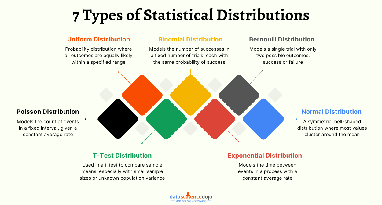
Statistical distributions help us understand a problem better by assigning a range of possible values to the variables, making them very useful in data science and machine learning. Here are 7 types of distributions with intuitive examples that often occur in real-life data.
Whether you’re guessing if it’s going to rain tomorrow, betting on a sports team to win an away match, framing a policy for an insurance company, or simply trying your luck on blackjack at the casino, probability, and distributions come into action in all aspects of life to determine the likelihood of events.
If you’re interested in learning how these come to life in advanced applications, you might find our LLM Bootcamp to be a great resource to deepen your understanding.
Having a sound statistical background can be incredibly beneficial in the daily life of a data scientist. Probability is one of the main building blocks of data science and machine learning. While the concept of probability gives us mathematical calculations, statistical distributions help us visualize what’s happening underneath.
Level up your AI game: Dive deep into Large Language Models with us!

Learn about Retrieval Augmented Generation and its role in LLM applications
Having a good grip on statistical distribution makes exploring a new dataset and finding patterns within a lot easier. It helps us choose the appropriate machine-learning model to fit our data and speed up the overall process.
In this blog, we will be going over diverse types of data, the common distributions for each of them, and compelling examples of where they are applied in real life.
Before we proceed further, if you want to learn more about probability distribution, watch this video below:
Common Types of Data
Explaining various distributions becomes more manageable if we are familiar with the type of data they use. We encounter two different outcomes in day-to-day experiments: finite and infinite outcomes.
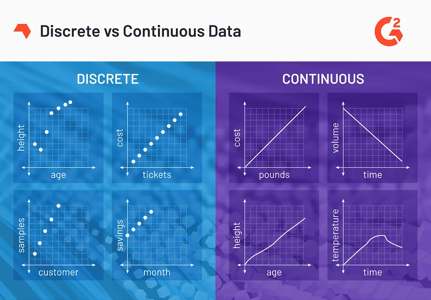
When you roll a die or pick a card from a deck, you have a limited number of outcomes possible. This type of data is called Discrete Data, which can only take a specified number of values. For example, in rolling a die, the specified values are 1, 2, 3, 4, 5, and 6.
Similarly, we can see examples of infinite outcomes from discrete events in our daily environment. Recording time or measuring a person’s height has infinitely many values within a given interval. This type of data is called Continuous Data, which can have any value within a given range. That range can be finite or infinite.
For example, suppose you measure a watermelon’s weight. It can be any value from 10.2 kg, 10.24 kg, or 10.243 kg. Making it measurable but not countable; hence, it is continuous. On the other hand, suppose you count the number of boys in a class; since the value is countable, it is discrete.
Types of Statistical Distributions
Depending on the type of data we use, we have grouped distributions into two categories, discrete distributions for discrete data (finite outcomes) and continuous distributions for continuous data (infinite outcomes).
Dig deeper into the Discrete vs Continuous data distributions
Discrete Distributions
Discrete Uniform Distribution: All Outcomes are Equally Likely
In statistics, uniform distribution refers to a statistical distribution in which all outcomes are equally likely. Consider rolling a six-sided die. You have an equal probability of obtaining all six numbers on your next roll, i.e., obtaining precisely one of 1, 2, 3, 4, 5, or 6, equaling a probability of 1/6, hence an example of a discrete uniform distribution.
As a result, the uniform distribution graph contains bars of equal height representing each outcome. In our example, the height is a probability of 1/6 (0.166667).
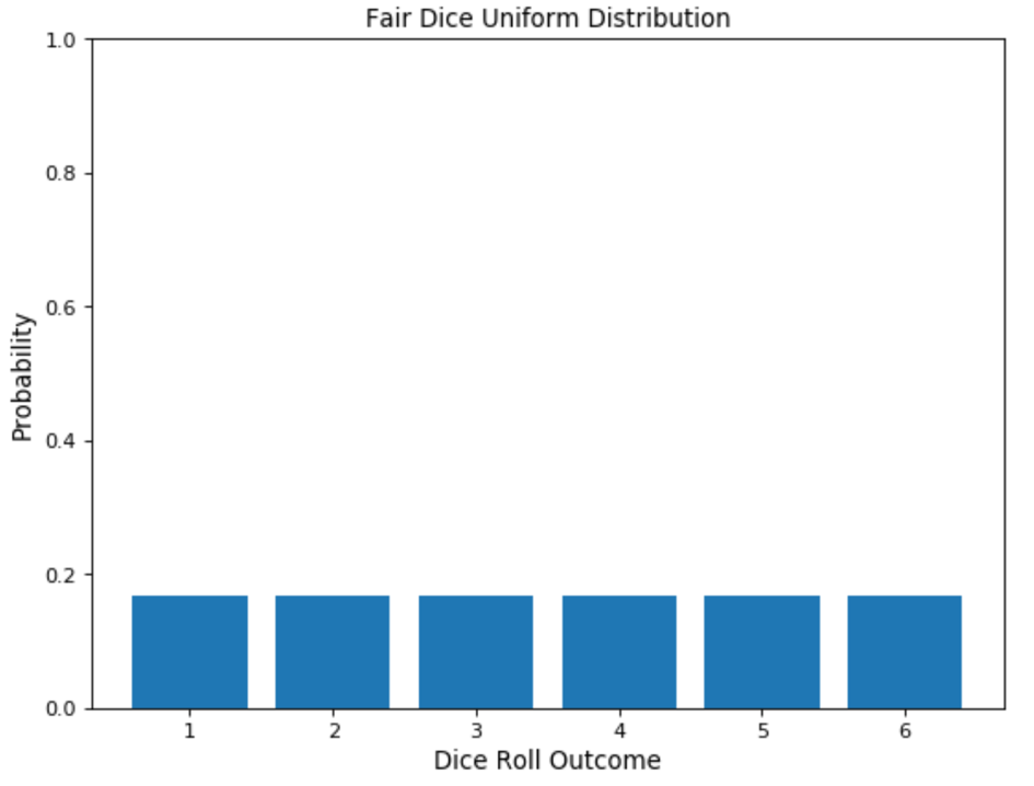
Uniform distribution is represented by the function U(a, b), where a and b represent the starting and ending values, respectively. Similar to a discrete uniform distribution, there is a continuous uniform distribution for continuous variables.
The drawbacks of this distribution are that it often provides us with no relevant information. Using our example of a rolling die, we get the expected value of 3.5, which gives us no accurate intuition since there is no such thing as half a number on a dice. Since all values are equally likely, it gives us no real predictive power.

Bernoulli Distribution: Single-trial with Two Possible Outcomes
The Bernoulli distribution is one of the easiest distributions to understand. It can be used as a starting point to derive more complex distributions. Any event with a single trial and only two outcomes follows a Bernoulli distribution. Flipping a coin or choosing between True and False in a quiz are examples of a Bernoulli distribution.
They have a single trial and only two outcomes. Let’s assume you flip a coin once; this is a single trail. The only two outcomes are either heads or tails. This is an example of a Bernoulli distribution.
Usually, when following a Bernoulli distribution, we have the probability of one of the outcomes (p). From (p), we can deduce the probability of the other outcome by subtracting it from the total probability (1), represented as (1-p).
It is represented by bern(p), where p is the probability of success. The expected value of a Bernoulli trial ‘x’ is represented as, E(x) = p, and similarly, Bernoulli variance is, Var(x) = p(1-p).
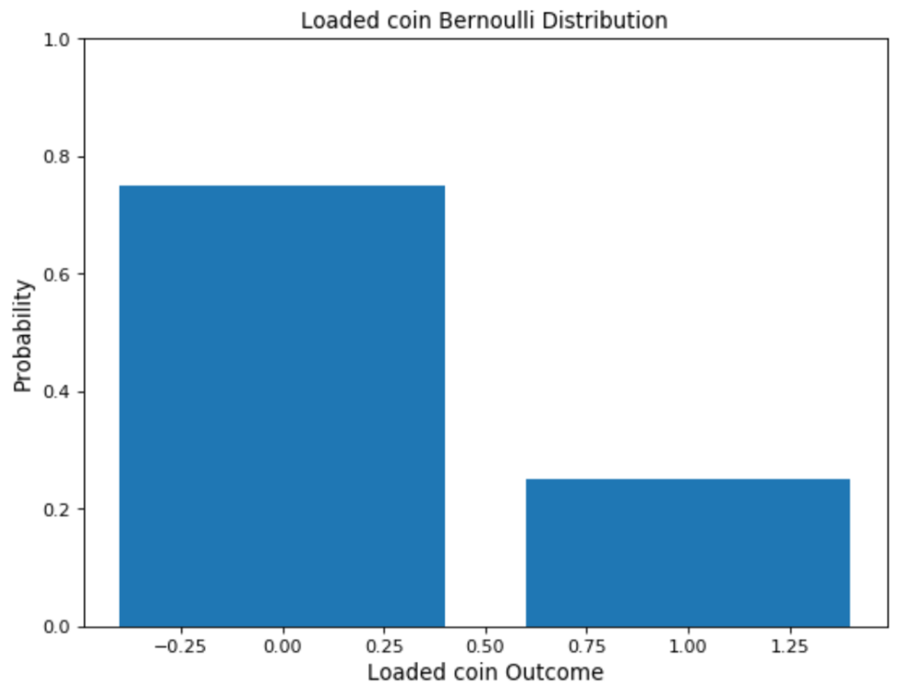
The graph of a Bernoulli distribution is simple to read. It consists of only two bars, one rising to the associated probability p and the other growing to 1-p.
Binomial Distribution: A Sequence of Bernoulli Events
The Binomial Distribution can be thought of as the sum of outcomes of an event following a Bernoulli distribution. Therefore, Binomial Distribution is used in binary outcome events, and the probability of success and failure is the same in all successive trials. An example of a binomial event would be flipping a coin multiple times to count the number of heads and tails.
Read more about Binomial Distribution and its importance in ML
Binomial vs Bernoulli distribution
The difference between these distributions can be explained through an example. Consider you’re attempting a quiz that contains 10 True/False questions. Trying a single T/F question would be considered a Bernoulli trial, whereas attempting the entire quiz of 10 T/F questions would be categorized as a Binomial trial. The main characteristics of Binomial Distribution are:
- Given multiple trials, each of them is independent of the other. That is, the outcome of one trial doesn’t affect another one.
- Each trial can lead to just two possible results (e.g., winning or losing), with probabilities p and (1 – p).
PRO TIP: Join our data science bootcamp program today to enhance your data science skillset!
A binomial distribution is represented by B (n, p), where n is the number of trials and p is the probability of success in a single trial. A Bernoulli distribution can be shaped as a binomial trial as B (1, p) since it has only one trial. The expected value of a binomial trial “x” is the number of times a success occurs, represented as E(x) = np. Similarly, variance is represented as Var(x) = np(1-p).
Let’s consider the probability of success (p) and the number of trials (n). We can then calculate the likelihood of success (x) for these n trials using the formula below:
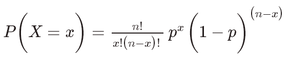
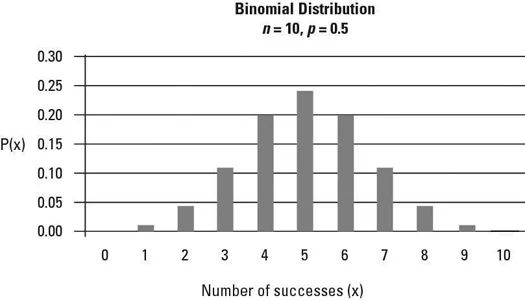
For example, suppose that a candy company produces both milk chocolate and dark chocolate candy bars. The total products contain half milk chocolate bars and half dark chocolate bars. Say you choose ten candy bars at random and choosing milk chocolate is defined as a success. The probability distribution of the number of successes during these ten trials with p = 0.5 is shown here in the binomial distribution graph:
Poisson Distribution: The Probability that an Event May or May not Occur
Poisson distribution deals with the frequency with which an event occurs within a specific interval. Instead of the probability of an event, Poisson distribution requires knowing how often it happens in a particular period or distance. For example, a cricket chirps two times in 7 seconds on average. We can use the Poisson distribution to determine the likelihood of it chirping five times in 15 seconds.
A Poisson process is represented with the notation Po(λ), where λ represents the expected number of events that can take place in a period. The expected value and variance of a Poisson process is λ. X represents the discrete random variable. A Poisson Distribution can be modeled using the following formula.
Understand more about the Poisson Process and its properties
The main characteristics which describe the Poisson Processes are:
- The events are independent of each other.
- An event can occur any number of times (within the defined period).
- Two events can’t take place simultaneously.
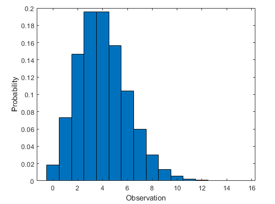
The graph of Poisson distribution plots the number of instances an event occurs in the standard interval of time and the probability of each one.
Continuous Distributions
Normal Distribution: Symmetric Distribution of Values Around the Mean
Normal distribution is the most used distribution in data science. In a normal distribution graph, data is symmetrically distributed with no skew. When plotted, the data follows a bell shape, with most values clustering around a central region and tapering off as they go further away from the center.
The normal distribution frequently appears in nature and life in various forms. For example, the scores of a quiz follow a normal distribution. Many of the students scored between 60 and 80 as illustrated in the graph below. Of course, students with scores that fall outside this range are deviating from the center.
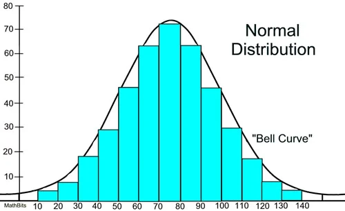
Here, you can witness the “bell-shaped” curve around the central region, indicating that most data points exist there. The normal distribution is represented as N(µ, σ2) here, µ represents the mean, and σ2 represents the variance, one of which is mostly provided. The expected value of a normal distribution is equal to its mean. Some of the characteristics which can help us to recognize a normal distribution are:
- The curve is symmetric at the center. Therefore mean, mode, and median are equal to the same value, distributing all the values symmetrically around the mean.
- The area under the distribution curve equals 1 (all the probabilities must sum up to 1).
Explore 9 key probability distributions in data science
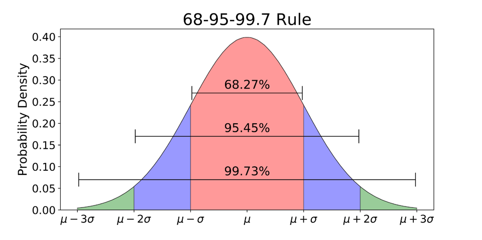
68-95-99.7 Rule
While plotting a graph for a normal distribution, 68% of all values lie within one standard deviation from the mean. In the example above, if the mean is 70 and the standard deviation is 10, 68% of the values will lie between 60 and 80. Similarly, 95% of the values lie within two standard deviations from the mean, and 99.7% lie within three standard deviations from the mean. This last interval captures almost all matters. If a data point is not included, it is most likely an outlier.
Student t-Test Distribution: Small Sample Size Approximation of a Normal Distribution
The student’s t-distribution, also known as the t distribution, is a type of statistical distribution similar to the normal distribution with its bell shape but has heavier tails. The t distribution is used instead of the normal distribution when you have small sample sizes.
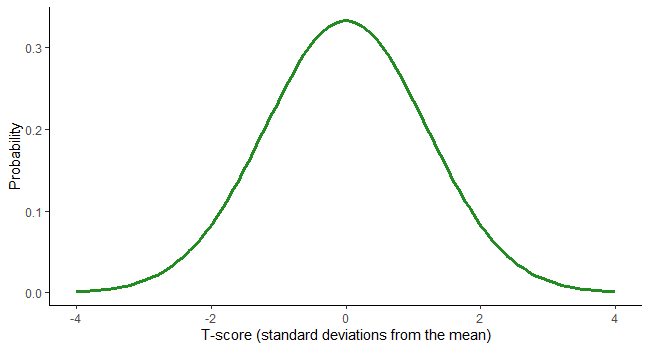
For example, suppose we deal with the total number of apples sold by a shopkeeper in a month. In that case, we will use the normal distribution. Whereas, if we are dealing with the total amount of apples sold in a day, i.e., a smaller sample, we can use the t distribution.
Read this blog to learn the top 7 statistical techniques for better data analysis
Another critical difference between the student’s t distribution and the Normal one is that apart from the mean and variance, we must also define the degrees of freedom for the distribution. In statistics, the number of degrees of freedom is the number of values in the final calculation of a statistic that are free to vary. A Student’s t distribution is represented as t(k), where k represents the number of degrees of freedom. For k=2, i.e., 2 degrees of freedom, the expected value is the same as the mean.
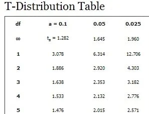
Degrees of freedom are in the left column of the t-distribution table.
Overall, the student t distribution is frequently used when conducting statistical analysis and plays a significant role in performing hypothesis testing with limited data.
Exponential Distribution: Model Elapsed Time between Two Events
Exponential distribution is one of the widely used continuous distributions. It is used to model the time taken between different events.
For example, in physics, it is often used to measure radioactive decay; in engineering, to measure the time associated with receiving a defective part on an assembly line; and in finance, to measure the likelihood of the next default for a portfolio of financial assets. Another common application of Exponential distributions in survival analysis (e.g., expected life of a device/machine).
Read the top 10 Statistics books to learn about Statistics
The exponential distribution is commonly represented as Exp(λ), where λ is the distribution parameter, often called the rate parameter. We can find the value of λ by the formula = 1/μ, where μ is the mean. Here, the standard deviation is the same as the mean. Var (x) gives the variance = 1/λ2
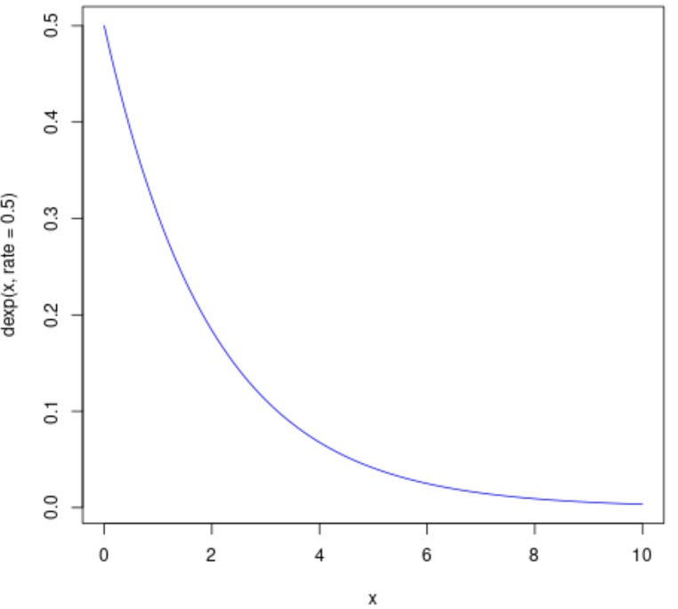
An exponential graph is a curved line representing how the probability changes exponentially. Exponential distributions are commonly used in calculations of product reliability or the length of time a product lasts.
Conclusion
Data is an essential component of the data exploration and model development process. The first thing that springs to mind when working with continuous variables is looking at the data distribution. We can adjust our machine-learning models to best match the problem if we can identify the pattern in the data distribution, which reduces the time to get to an accurate outcome.

Indeed, specific Machine Learning models are built to perform best when certain distribution assumptions are met. Knowing which distributions, we’re dealing with may thus assist us in determining which models to apply.