

Statistical distributions help us understand a problem better by assigning a range of possible values to the variables, making them very useful in data science and machine learning. Here are 6 types of distributions with intuitive examples that often occur in real-life data.
In statistics, a distribution is simply a way to understand how a set of data points are spread over some given range of values.
For example, distribution takes place when the merchant and the producer agree to sell the product during a specific time frame. This form of distribution is exhibited by the agreement reached between Apple and AT&T to distribute their products in the United States.
Types of statistical distributions
There are several statistical distributions, each representing different types of data and serving different purposes. Here we will cover several commonly used distributions.
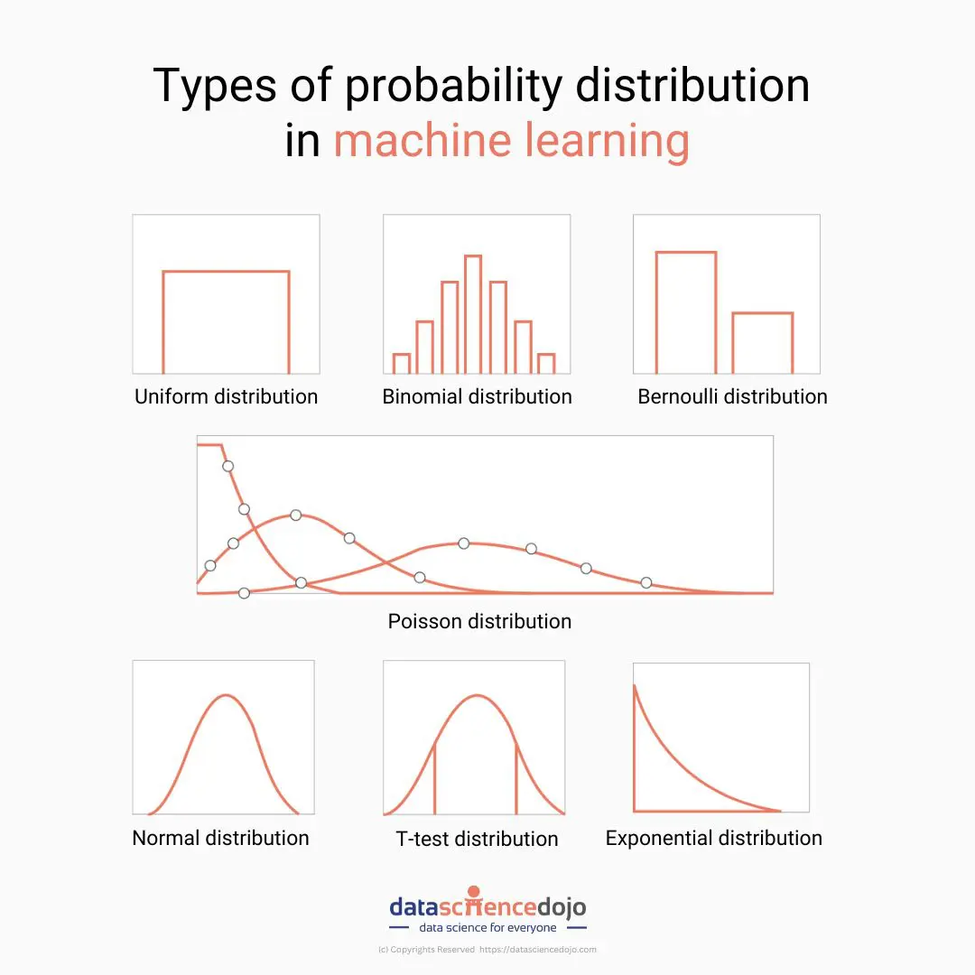
- Normal Distribution
- t-Distribution
- Binomial Distribution
- Poisson Distribution
- Uniform Distribution
Pro-tip: Enroll in the data science bootcamp today and advance your learning
1. Normal Distribution
A normal distribution also known as “Gaussian Distribution” shows the probability density for a population of continuous data (for example height in cm for all NBA players). Also, it indicates the likelihood that any NBA player will have a particular height. Let’s say fewer players are much taller or shorter than usual; most are close to average height.
The spread of the values in our population is measured using a metric called standard deviation. The Empirical Rule tells us that:
- 68.3% of the values will fall between1 standard deviation above and below the mean
- 95.5% of the values will fall between2 standard deviations above and below the mean
- 99.7% of the values will fall between3 standard deviations above and below the mean
Let’s assume that we know that the mean height of all players in the NBA is 200cm and the standard deviation is 7cm. If Le Bron James is 206 cm tall, what proportion of NBA players is he taller than? We can figure this out! LeBron is 6cm taller than the mean (206cm – 200cm). Since the standard deviation is 7cm, he is 0.86 standard deviations (6cm / 7cm) above the mean.
Our value of 0.86 standard deviations is called the z-score. This shows that James is taller than 80.5% of players in the NBA!
This can be converted to a percentile using the probability density function (or a look-up table) giving us our answer. A probability density function (PDF) defines the random variable’s probability of coming within a distinct range of values.
2. t-distribution
A t-distribution is symmetrical around the mean, like a normal distribution, and its breadth is determined by the variance of the data. A t-distribution is made for circumstances where the sample size is limited, but a normal distribution works with a population. With a smaller sample size, the t-distribution takes on a broader range to account for the increased level of uncertainty.
The number of degrees of freedom, which is determined by dividing the sample size by one, determines the curve of a t-distribution. The t-distribution tends to resemble a normal distribution as sample size and degrees of freedom increase because a bigger sample size increases our confidence in estimating the underlying population statistics.
For example, suppose we deal with the total number of apples sold by a shopkeeper in a month. In that case, we will use the normal distribution. Whereas, if we are dealing with the total amount of apples sold in a day, i.e., a smaller sample, we can use the t distribution.
3. Binomial distribution
A Binomial Distribution can look a lot like a normal distribution’s shape. The main difference is that instead of plotting continuous data, it plots a distribution of two possible discrete outcomes, for example, the results from flipping a coin. Imagine flipping a coin 10 times, and from those 10 flips, noting down how many were “Heads”. It could be any number between 1 and 10. Now imagine repeating that task 1,000 times.
If the coin, we are using is indeed fair (not biased to heads or tails) then the distribution of outcomes should start to look at the plot above. In the vast majority of cases, we get 4, 5, or 6 “heads” from each set of 10 flips, and the likelihood of getting more extreme results is much rarer!
4. Bernoulli distribution
The Bernoulli Distribution is a special case of Binomial Distribution. It considers only two possible outcomes, success, and failure, true or false. It’s a really simple distribution, but worth knowing! In the example below we’re looking at the probability of rolling a 6 with a standard die.
If we roll a die many, many times, we should end up with a probability of rolling a 6, 1 out of every 6 times (or 16.7%) and thus a probability of not rolling a 6, in other words rolling a 1,2,3,4 or 5, 5 times out of 6 (or 83.3%) of the time!
5. Discrete uniform distribution: All outcomes are equally likely
Uniform distribution is represented by the function U(a, b), where a and b represent the starting and ending values, respectively. Like a discrete uniform distribution, there is a continuous uniform distribution for continuous variables.
In statistics, uniform distribution refers to a statistical distribution in which all outcomes are equally likely. Consider rolling a six-sided die. You have an equal probability of obtaining all six numbers on your next roll, i.e., obtaining precisely one of 1, 2, 3, 4, 5, or 6, equaling a probability of 1/6, hence an example of a discrete uniform distribution.
As a result, the uniform distribution graph contains bars of equal height representing each outcome. In our example, the height is a probability of 1/6 (0.166667).
The drawbacks of this distribution are that it often provides us with no relevant information. Using our example of a rolling die, we get the expected value of 3.5, which gives us no accurate intuition since there is no such thing as half a number on a dice. Since all values are equally likely, it gives us no real predictive power.
It is a distribution in which all events are equally likely to occur. Below, we’re looking at the results from rolling a die many, many times. We’re looking at which number we got on each roll and tallying these up. If we roll the die enough times (and the die is fair) we should end up with a completely uniform probability where the chance of getting any outcome is exactly the same
6. Poisson distribution
A Poisson Distribution is a discrete distribution similar to the Binomial Distribution (in that we’re plotting the probability of whole numbered outcomes) Unlike the other distributions we have seen however, this one is not symmetrical – it is instead bounded between 0 and infinity.
For example, a cricket chirps two times in 7 seconds on average. We can use the Poisson distribution to determine the likelihood of it chirping five times in 15 seconds. A Poisson process is represented with the notation Po(λ), where λ represents the expected number of events that can take place in a period.
The expected value and variance of a Poisson process is λ. X represents the discrete random variable. A Poisson Distribution can be modeled using the following formula.
The Poisson distribution describes the number of events or outcomes that occur during some fixed interval. Most commonly this is a time interval like in our example below where we are plotting the distribution of sales per hour in a shop.
Conclusion:
Data is an essential component of the data exploration and model development process. We can adjust our Machine Learning models to best match the problem if we can identify the pattern in the data distribution, which reduces the time to get to an accurate outcome.
Indeed, specific Machine Learning models are built to perform best when certain distribution assumptions are met. Knowing which distributions, we’re dealing with may thus assist us in determining which models to apply.