

Probability distributions are fundamental to data science, influencing the ways in which we analyze and interpret data. They offer a systematic approach to modeling uncertainty, facilitating predictions, and extracting insights from real-world events.

Whether it’s understanding customer behavior or refining machine learning models, probability distributions are crucial in the decision-making process. In this blog, we will delve into nine fundamental probability distributions commonly used in data science
Whether you’re new to the field or a seasoned data scientist, gaining expertise in these distributions will significantly improve your data analysis skills. In the realm of data science, understanding probability distributions is crucial. They provide a mathematical framework for modeling and analyzing data.
Understand the applications of probability in data science
Explore Probability Distributions in Data Science with Practical Applications
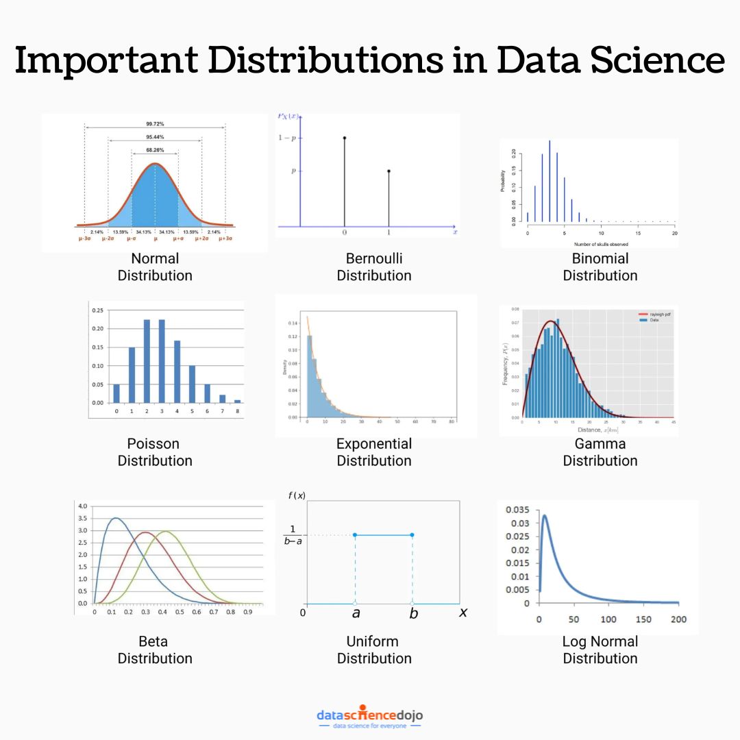
Following are the nine important data science distributions and their practical applications:
1. Normal Distribution
The normal distribution, characterized by its bell-shaped curve, is prevalent in various natural phenomena. For instance, IQ scores in a population tend to follow a normal distribution. This allows psychologists and educators to understand the distribution of intelligence levels and make informed decisions regarding education programs and interventions.
Learn how AI is empowering the education industry
Heights of adult males in a given population often exhibit a normal distribution. In such a scenario, most men tend to cluster around the average height, with fewer individuals being exceptionally tall or short.
This means that the majority fall within one standard deviation of the mean, while a smaller percentage deviates further from the average.
2. Binomial Distribution
The binomial distribution describes the number of successes in a fixed number of Bernoulli trials. Imagine conducting 10 coin flips and counting the number of heads. This scenario follows a binomial distribution. In practice, this distribution is used in fields like manufacturing, where it helps in estimating the probability of defects in a batch of products.
Imagine a basketball player with a 70% free throw success rate. If this player attempts 10 free throws, the number of successful shots follows a binomial distribution. This distribution allows us to calculate the probability of making a specific number of successful shots out of the total attempts.
3. Bernoulli Distribution
The Bernoulli distribution models a random variable with two possible outcomes: success or failure. Consider a scenario where a coin is tossed. Here, the outcome can be either a head (success) or a tail (failure). This distribution finds application in various fields, including quality control, where it’s used to assess whether a product meets a specific quality standard.
When flipping a fair coin, the outcome of each flip can be modeled using a Bernoulli distribution. This distribution is aptly suited as it accounts for only two possible results – heads or tails. The probability of success (getting a head) is 0.5, making it a fundamental model for simple binary events.
4. Poisson Distribution
The Poisson distribution models the number of events occurring in a fixed interval of time or space, assuming a constant rate. For example, in a call center, the number of calls received in an hour can often be modeled using a Poisson distribution. This information is crucial for optimizing staffing levels to meet customer demands efficiently.
Learn about 5 tips to enhance customer service using data science
In the context of a call center, the number of incoming calls over a given period can often be modeled using a Poisson distribution. This distribution is applicable when events occur randomly and are relatively rare, like calls to a hotline or requests for customer service during specific hours.
5. Exponential Distribution
The exponential distribution represents the time until a continuous, random event occurs. In the context of reliability engineering, this distribution is employed to model the lifespan of a device or system before it fails. This information aids in maintenance planning and ensuring uninterrupted operation.
The time intervals between successive earthquakes in a certain region can be accurately modeled by an exponential distribution. This is especially true when these events occur randomly over time, but the probability of them happening in a particular time frame is constant.
6. Gamma Distribution
The gamma distribution extends the concept of the exponential distribution to model the sum of k independent exponential random variables. This distribution is used in various domains, including queuing theory, where it helps in understanding waiting times in systems with multiple stages.
Consider a scenario where customers arrive at a service point following a Poisson process, and the time it takes to serve them follows an exponential distribution. In this case, the total waiting time for a certain number of customers can be accurately described using a gamma distribution. This is particularly relevant for modeling queues and wait times in various service industries.

7. Beta Distribution
The beta distribution is a continuous probability distribution bound between 0 and 1. It’s widely used in Bayesian statistics to model probabilities and proportions. In marketing, for instance, it can be applied to optimize conversion rates on a website, allowing businesses to make data-driven decisions to enhance user experience.
In the realm of A/B testing, the conversion rate of users interacting with two different versions of a webpage or product is often modeled using a beta distribution. This distribution allows analysts to estimate the uncertainty associated with conversion rates and make informed decisions regarding which version to implement.
8. Uniform Distribution
In a uniform distribution, all outcomes have an equal probability of occurring. A classic example is rolling a fair six-sided die. In simulations and games, the uniform distribution is used to model random events where each outcome is equally likely.
When rolling a fair six-sided die, each outcome (1 through 6) has an equal probability of occurring. This characteristic makes it a prime example of a discrete uniform distribution, where each possible outcome has the same likelihood of happening.
Get started with your data science learning journey with our instructor-led live bootcamp. Explore now.
9. Log Normal Distribution
The log normal distribution describes a random variable whose logarithm is normally distributed. In finance, this distribution is applied to model the prices of financial assets, such as stocks. Understanding the log normal distribution is crucial for making informed investment decisions.
The distribution of wealth among individuals in an economy often follows a log-normal distribution. This means that when the logarithm of wealth is considered, the resulting values tend to cluster around a central point, reflecting the skewed nature of wealth distribution in many societies.
Learn Probability Distributions Today!
Understanding these distributions and their applications empowers data scientists to make informed decisions and build accurate models. Remember, the choice of distribution greatly impacts the interpretation of results, so it’s a critical aspect of data analysis.
Delve deeper into probability with this short tutorial
Final Thoughts
Getting a solid grasp of probability distributions is key to making sense of data and creating reliable models in data science. Each type of distribution has its own unique role—whether it’s capturing natural patterns with the normal distribution or forecasting rare occurrences with the Poisson distribution.
By mastering these tools, data scientists can make smarter decisions, fine-tune algorithms, and improve real-world outcomes.

As you dive deeper into your data science journey, keep exploring these distributions and how they’re applied in practice. The more you understand them, the stronger and more impactful your data-driven insights will become!