

This blog explores the important steps one should follow in the data preprocessing stage such as eradicating duplicates, fixing structural errors, detecting, and handling outliers, type conversion, dealing with missing values, and data encoding.
What is data preprocessing?
A common mistake that many novice data scientists make is that they skip through the data wrangling stage and dive right into the model-building phase, which in turn generates a poor-performing machine learning model.
This resembles a popular concept in the field of data science called GIGO (Garbage in Garbage Out). This concept means inferior quality data will always yield poor results irrespective of the model and optimization technique used.
Hence, an ample amount of time needs to be invested in ensuring the quality of the data is up to standard. In fact, data scientists spend around 80% of their time just on the data pre-processing phase.
But fret not, because we will investigate the various steps that you can follow to ensure that your data is preprocessed before stepping ahead in the data science pipeline.

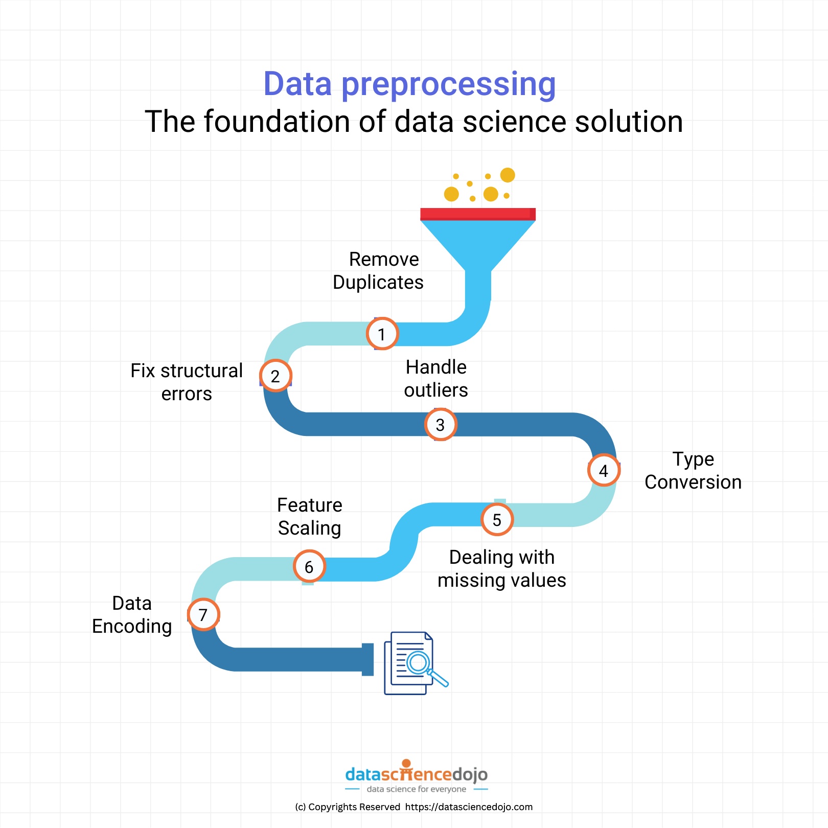
Let’s look at the steps of data pre-processing to understand it better:
Removing duplicates:
You may often encounter repeated entries in your dataset, which is not a good sign because duplicates are an extreme case of non-random sampling, and they tend to make the model biased. Including repeated entries will lead to the model overfitting this subset of points and hence must be removed.
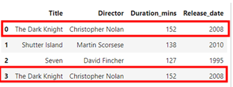
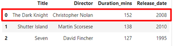
We will demonstrate this with the help of an example. Let’s say we had a movie data set as follows:
As we can see, the movie title “The Dark Knight” is repeated at the 3rd index (fourth entry) in the data frame and needs to be taken care of.
Using the code below, we can remove the duplicate entries from the dataset based on the “Title” column and only keep the first occurrence of the entry.
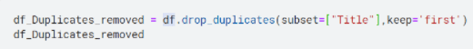
Just by writing a few lines of code, you ensure your data is free from any duplicate entries. That’s how easy it is!
Fix structural errors:
Structural errors in a dataset refer to the entries that either have typos or inconsistent spellings:
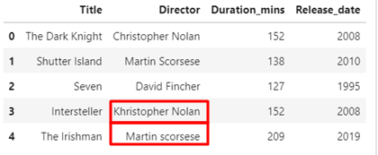
Here, you can easily spot the different typos and inconsistencies, but what if the dataset was huge? You can check all the unique values and their corresponding occurrences using the following code:
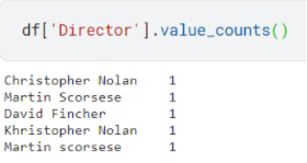
Once you identify the entries to be fixed, simply replace the values with the correct version.
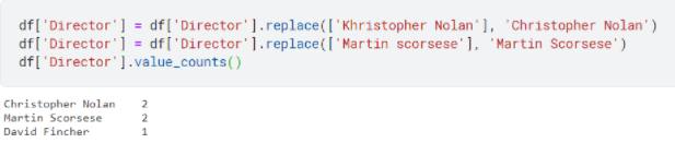
Voila! That is how you fix the structural errors.
Detecting and handling outliers:
Before we dive into detecting and handling outliers, let’s discuss what an outlier is.
“Outlier is any value in a dataset that drastically deviates from the rest of the data points.”
Let’s say we have a dataset of a streaming service with the ages of users ranging from 18 to 60, but there exists a user whose age is registered as 200. This data point is an example of an outlier and can mess up our machine-learning model if not taken care of.

There are numerous techniques that can be employed to detect and remove outliers in a data set but the ones that I am going to discuss are:
- Box plots
- Z- Score
Let’s assume the following data set:
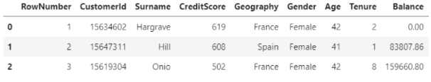
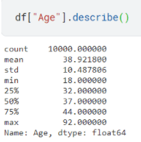
If we use the describe function of pandas on the Age column, we can analyze the five number summary along with count, mean, and standard deviation of the specified column, then by using the domain specific knowledge like for the above instance we know that significantly large values of age can be a result of human error we can deduce that there are outliers in the dataset as the mean is 38.92 while the max value is 92.
As we have got some idea about what outliers are, let’s see some code in action to detect and remove the outliers
Box Plots:
Box plots or also called “Box and Whiskers Plot” show the five number summary of the features under consideration and are an effective way of visualizing the outlier.
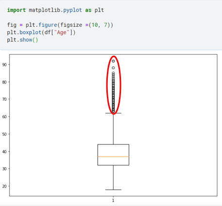
As we can see from the above figure, there are number of data points that are outliers. So now we move onto Z-Score, a method through which we are going to set the threshold and remove the outlier entries from our dataset.
Z- Score:
A z-score determines the position of a data point in terms of its distance from the mean when measured in standard deviation units.
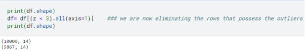
We first calculate the Z-score of the feature column:
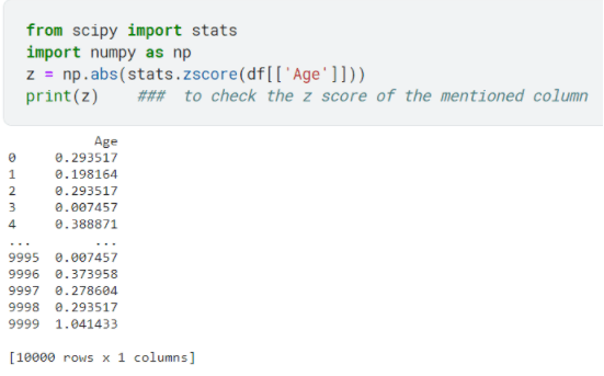
The standard normal curve (Z-score) for a set of values represents 99.7% of the data points within the range of –3 and +3 scores, so in practice often the threshold is set to be 3 and anything beyond that is deemed an outlier and hence removed from the dataset if problematic or not a legitimate observation.
Type Conversion:
Type conversion refers to when certain columns are not of valid data type, for instance, in the following data frame, three out of four columns are of object data type:
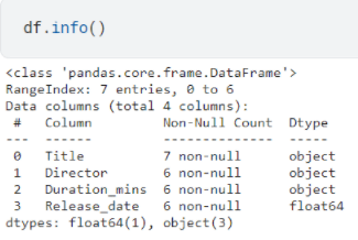
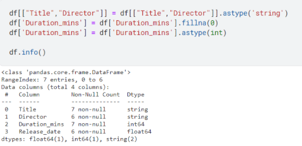
Well, we don’t want that right? Because it would produce unexpected results and errors. We are going to convert Title and Director to string data types, and Duration_mins to integer data type.
- Dealing With Missing Values:
Often, data set contains numerous missing values, which can be a problem. To name a few it can play a role in development of biased estimator, or it can decrease the representativeness of the sample under consideration.
Which brings us to the question of how to deal with them.
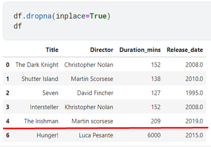
One thing you could do is simply drop them all. If you notice that index 5 has a few missing values, when the “dropna” command is implemented, it will drop that row from the dataset.
But what to do when you have a limited number of rows in a dataset? You could use different imputations methods such as the Measures of central tendencies to fill those empty cells.
The measures include:
- Mean: The mean is the average of a data set. It is “sensitive” to outliers.
- Median: The median is the middle of the set of numbers. It is resistant to outliers
- Mode: The mode is the most common number in a data set.
It is better to use median instead of mean because of the property of not deviating drastically because of outliers. Allow me to elaborate this with an example
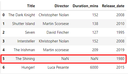
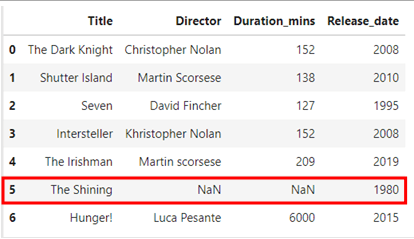
Notice how there is a documentary by the name “Hunger!” with “Duration_mins” equal to 6000 now observe the difference when I replace the missing value in the duration column with mean and with median.
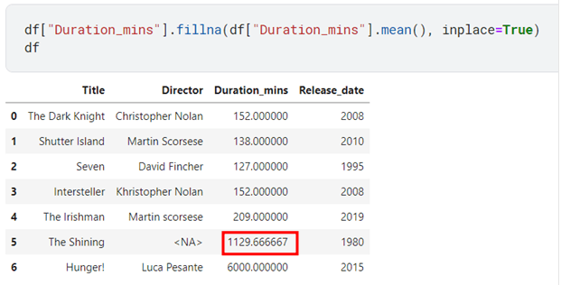
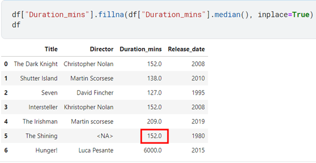
If you search on the internet for the duration of movie “The Shining” you’ll find out it’s about 146 minutes so, isn’t 152 minutes much closer as compared to 1129 as calculated by mean?
A few other techniques to fill the missing values that you can explore are forward fill and backward fill.
Forward will work on the principle that the last valid value of a column is passed forward to the missing cell of the dataset.
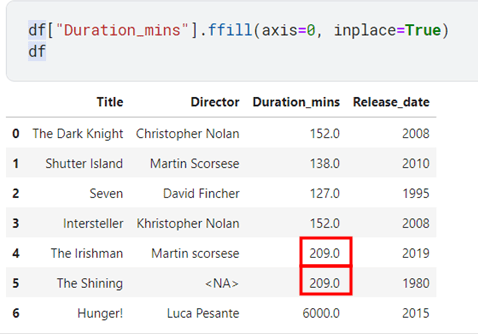
Notice how 209 propagated forward.
Let’s observe backward fill too
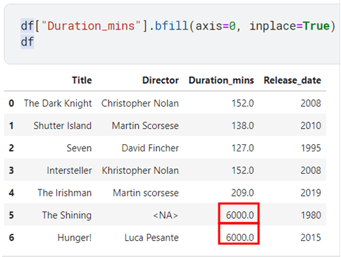
From the above example, you can clearly see that the value following the empty cell was propagated backwards to fill in that missing cell.
The final technique I’m going to show you is called linear interpolation. What we do is take the mean of the values prior to and following the empty cell and use it to fill in the missing value.
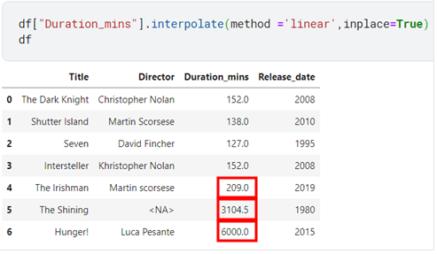
3104.5 is the mean of 209 and 6000. As you can see this technique is too affected by outliers.
That was a quick run-down on how to handle missing values, moving onto the next section.
Feature scaling:
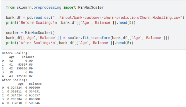
Another core concept of data preprocessing is the feature scaling of your dataset. In simple terms feature scaling refers to the technique where you scale multiple (quantitative) columns of your dataset to a common scale.
Assume a banking dataset has a column of age which usually ranges from 18 to 60 and a column of balance which can range from 0 to 10000. If you observe, there is an enormous difference between the values each data point can assume, and machine learning model would be affected by the balance column and would assign higher weights to it as it would consider the higher magnitude of balance to carry more importance as compared to age which has relatively lower magnitude.
To rectify this, we use the following two methods:
- Normalization
- Standardization
Normalization fits the data between the ranges of [0,1] but sometimes [-1,1] too. It is affected by outliers in a dataset and is useful when you do not know about the distribution of dataset.
Standardization, on the other hand, is not bound to be within a certain range; it’s quite resistant to outliers and useful when the distribution is normal or Gaussian.
Normalization:
Standardization:

Data encoding
The last step of the data preprocessing stage is the data encoding. It is where you encode the categorical features (columns) of your dataset into numeric values.
There are many encoding techniques available, but I’m just going to show you the implementation of one hot encoding (Pro-tip: You should use this when the order of the data does not matter).
For instance, in the following example, the gender column is nominal data, meaning that the identification of your gender does not take precedence over other genders. To further clarify the concept, let’s assume, for the sake of argument, we had a dataset of examination results of some high school class with a column of rank. The rank here is an example of ordinal data as it would follow a certain order and higher-ranking students would take precedence over lower-ranked ones.
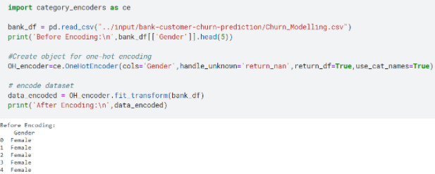
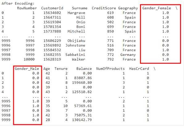
If you notice in the above example, the gender column could assume one of the two options that were either male or female. What one hot encoder did was create the same number of columns as the number of options available, then for the row that had the associated possible value encode it with one (why one?). Well because one is the binary representation of true) otherwise zero (you guessed, zero represents false)
If you do wish to explore other techniques, here is an excellent resource for this purpose:
Blog: Types of categorical data encoding
Conclusion:
It might have been a lot to take in, but you have now explored the crucial concept of data science, that is data preprocessing.; Moreover, you are now equipped with the steps to curate your dataset in such a way that it will yield satisfactory results.
The journey to becoming a data scientist can seem daunting, but with the right mentorship, you can learn it seamlessly and take on real world problems in no time, to embark on the journey of becoming a data scientist, enroll yourself in the Data Science bootcamp and grow your career.