Shehryar Mallick

This blog explores the amazing (Artificial Intelligence) AI technology called ChatGPT that has taken the world by storm and tries to unravel the underlying phenomenon that makes up this seemingly complex technology.

What is ChatGPT? 

ChatGPT was officially launched on 30th November 2022 by OpenAI and quickly amassed a huge following not even in a week. Just to give you an idea it took Facebook around 10 months to gain 1 million followers ChatGPT did it in 5 days. So, the question that might arise in your minds my dear readers is why? Why did it gain so much popularity? What purpose does it serve? How does it work? Well, fret not we are here to answer those questions in this blog. 

Let us begin by understanding what ChatGPT is, ChatGPT is a language model that uses reinforcement learning from human feedback (RLHF) to keep on learning and fine-tuning its responses, it can answer a wide variety of questions within a span of a few minutes, help you in numerous tasks by giving you a curated, targeted response rather than vague links in a human-like manner. 

Be it writing a code or searching for something chances are ChatGPT already has the specific thing you are looking for. This brings us to our next question; how does it work? Is there magic behind it? No, it is just the clever use of machine learning and an abundance of use cases and data that OpenAI created something as powerful and elegant as ChatGPT. 

The architecture of Chat GPT 

ChatGPT is a variant of transformer-based neural network architecture, introduced in a paper by the name “Attention is all you need” in 2017, transformer architecture was specifically designed for NLP (Natural Language Processing) tasks and prevails as one of the most used methods to date. 

A quick overview of the architecture involves its usage of self-attention mechanisms which allow the model to focus on specific words and phrases when generating text, rather than processing the entire input as a single unit. It consists of multiple layers, each of which contains a multi-head self-attention mechanism and a fully connected neural network.

Also, it includes a mechanism called positional encoding which lets the model understand the relative position of the words in the input. This architecture has proven to be amazingly effective in natural language processing tasks such as text generation, language translation, and text summarization.

Following are the different layers that are involved in the architecture of ChatGPT 

• An embedding layer: this layer is responsible for converting the input words into a dense vector representation that the model can process. 
• Multiple layers of self-attention: these layers are responsible for analyzing the input and calculating a set of attention weights, which indicate which parts of the input are most important for the current task. 
• Multi-head attention: this layer is responsible for concatenating the outputs of multiple self-attention layers and then linearly transforming the resulting concatenated vectors 
• Multiple layers of fully connected neural networks: these layers are responsible for transforming the output of the attention layers into a final representation that can be used for the task at hand. 
• Output layer: this layer is responsible for generating the final output of the model, which can be a probability distribution over the possible next words in a sentence or a classification label for a given input text
   

Flow of ChatGPT

After getting a basic understanding of what ChatGPT is and its internal architecture we will now see the flow of ChatGPT from the training phase to answering a user prompt. 

1. Data collection:

Around 300 billion words were gathered for the training of ChatGPT, the sources for the data mainly included books, articles, and websites. 

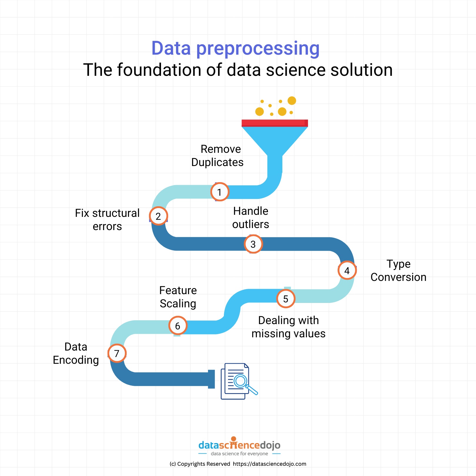
2. Pre-Processing:

Once the data was collected it needed to be preprocessed so that it could be used for training. Techniques involved in preprocessing are stopped word removal, removal of duplicate data, lowercasing, removing special characters, tokenization, etc. 

3. Training:

The pre-processed data is used to train ChatGPT, which is a variant of the transformer architecture. During training, the model learns the patterns and relationships between words, phrases, and sentences. This process can take several days to several weeks depending on the size of the dataset and the computational resources available. 

4. Fine-tuning:

Once the pre-training is done, the model can be fine-tuned on a smaller, task-specific data set to improve its performance on specific natural language processing tasks. 

5. Inference:

The trained and fine-tuned model is ready to generate responses to prompts. The input prompt is passed through the model, which uses its pre-trained weights and the patterns it learned during the training phase to generate a response. 

6. Output:

The model generates a final output, which is a sequence of words that forms the answer to the prompt. 

Strengths of the AI technology of ChatGPT

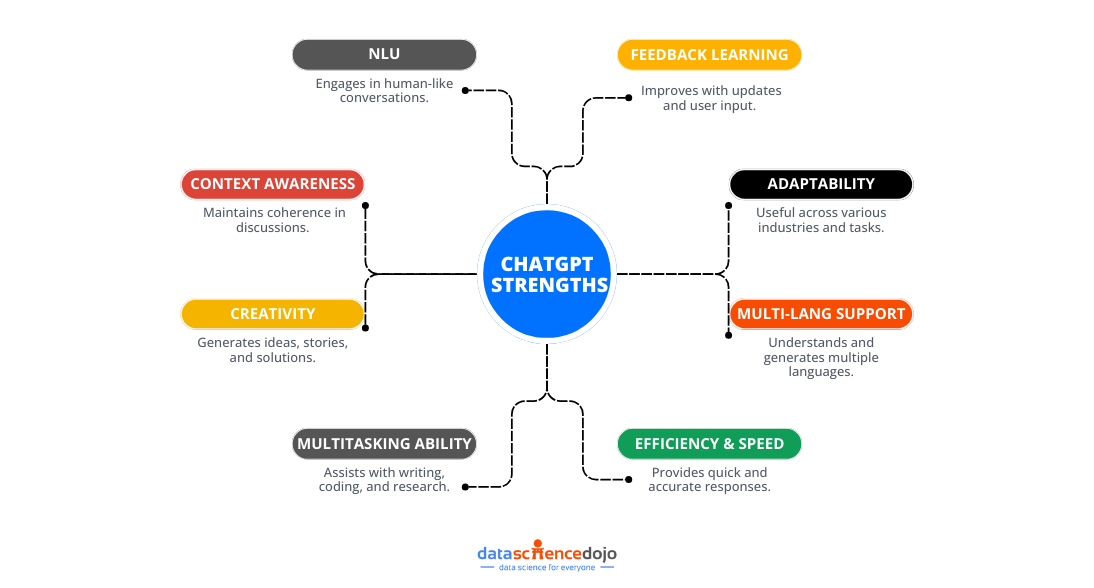
• ChatGPT is a large language model that has been trained on a massive dataset of text data, allowing it to understand and generate human-like text. 
• It can perform a wide range of natural language processing tasks such as text completion, question answering, and conversation simulation. 
• The transformer-based neural network architecture enables ChatGPT to understand the context of the input and generate a response accordingly. 
• It can handle large input sequences and generate coherent and fluent text; this makes it suitable for long-form text generation tasks. 
• ChatGPT can be used for multiple languages and can be fine-tuned for different dialects and languages. 
• It can be easily integrated with other NLP tasks, such as named entity recognition, sentiment analysis, and text summarization 
• It can also be used in several applications like chatbots, virtual assistants, and language model-based text generation tasks.
   

Weaknesses of ChatGPT

• ChatGPT is limited by the information contained in the training data and does not have access to external knowledge, which may affect its ability to answer certain questions. 
• The model can be exposed to biases and stereotypes present in the training data, so the generated text should be used with caution. 
• ChatGPT’s performance on languages other than English may be limited. 
• Training and running ChatGPT requires significant computational resources and memory. 
• ChatGPT is limited to natural language processing tasks and cannot perform tasks such as image or speech recognition. 
• Lack of common-sense reasoning ability: ChatGPT is a language model and lacks the ability to understand common-sense reasoning, which can make it difficult to understand some context-based questions. 
• Lack of understanding of sarcasm and irony: ChatGPT is trained on text data, which can lack sarcasm and irony, so it might not be able to understand them in the input. 
• Privacy and security concerns: ChatGPT and other similar models are trained on large amounts of text data, which may include sensitive information, and the model’s parameters can also be used to infer sensitive information about the training data. 

 

Storming the Internet – What’s Chat GPT-4?

The latest development in artificial intelligence (AI) has taken the internet by storm. OpenAI’s new language model, GPT-4, has everyone talking. GPT-4 is an upgrade from its predecessor, GPT-3, which was already an impressive language model. GPT-4 has improved capabilities, and it is expected to be even more advanced and powerful.

With GPT-4, there is excitement about the potential for advancements in natural language processing, which could lead to breakthroughs in many fields, including medicine, finance, and customer service. GPT-4 could enable computers to understand natural language more effectively and generate more human-like responses.

A glimpse into Auto GPT

However, it is not just GPT-4 that is causing a stir. Other AI language models, such as Auto GPT, are also making waves in the tech industry. Auto GPT is a machine learning system that can generate text on its own without any human intervention. It has the potential to automate content creation for businesses, making it a valuable tool for marketers.

Auto chat is particularly useful for businesses that need to engage with customers in real-time, such as customer service departments. By using auto chat, companies can reduce wait times, improve response accuracy and provide a more personalized customer experience.

Want to start your EDA journey, well you can always get yourself registered at Data Science Bootcamp.

In a nutshell

So just to recap, ChatGPT is not a black box of unknown mysteries but rather a carefully crafted state-of-the-art artificial intelligence algorithm that has been rigorously trained with a variety of scenarios in order to cover all the possible use cases. Even though it can do wonders as we have seen already there is still a long way to go as there are still potential problems that need to be inspected and worked on. To get the latest news on astounding technological advancements and other associated fields visit Data Science Dojo to keep yourself posted.   

 

ChatGPT is scary good. We are not far from dangerously strong AI – Elon Musk  

This blog explores the difference between mutable and immutable objects in Python. 

Python is a powerful programming language with a wide range of applications in various industries. Understanding how to use mutable and immutable objects is essential for efficient and effective Python programming. In this guide, we will take a deep dive into mastering mutable and immutable objects in Python.

Mutable objects

In Python, an object is considered mutable if its value can be changed after it has been created. This means that any operation that modifies a mutable object will modify the original object itself. To put it simply, mutable objects are those that can be modified either in terms of state or contents after they have been created. The mutable objects that are present in python are lists, dictionaries and sets. 

 

 

 

Advantages of mutable objects 

• They can be modified in place, which can be more efficient than recreating an immutable object. 
• They can be used for more complex and dynamic data structures, like lists and dictionaries. 

Disadvantages of mutable objects 

• They can be modified by another thread, which can lead to race conditions and other concurrency issues. 
• They can’t be used as keys in a dictionary or elements in a set. 
• They can be more difficult to reason about and debug because their state can change unexpectedly.

Want to start your EDA journey? Well you can always get yourself registered at Python for Data Science.

While mutable objects are a powerful feature of Python, they can also be tricky to work with, especially when dealing with multiple references to the same object. By following best practices and being mindful of the potential pitfalls of using mutable objects, you can write more efficient and reliable Python code.

Immutable objects 

In Python, an object is considered immutable if its value cannot be changed after it has been created. This means that any operation that modifies an immutable object returns a new object with the modified value. In contrast to mutable objects, immutable objects are those whose state cannot be modified once they are created. Examples of immutable objects in Python include strings, tuples, and numbers.

 

 

 

Advantages of immutable objects 

• They are safer to use in a multi-threaded environment as they cannot be modified by another thread once created, thus reducing the risk of race conditions. 
• They can be used as keys in a dictionary because they are hashable and their hash value will not change. 
• They can be used as elements of a set because they are comparable, and their value will not change. 
• They are simpler to reason about and debug because their state cannot change unexpectedly. 

Disadvantages of immutable objects

• They need to be recreated if their value needs to be changed, which can be less efficient than modifying the state of a mutable object. 
• They take up more memory if they are used in large numbers, as new objects need to be created instead of modifying the state of existing objects. 

 

In this blog, we will discuss exploratory data analysis, also known as EDA, and why it is important. We will also be sharing code snippets so you can try out different analysis techniques yourself. So, without any further ado let’s dive right in. 

What is Exploratory Data Analysis (EDA)? 

“The greatest value of a picture is when it forces us to notice what we never expected to see.”  John Tukey, American Mathematician 

A core skill to possess for someone who aims to pursue data science, data analysis or affiliated fields as a career is exploratory data analysis (EDA). To put it simply, the goal of EDA is to discover underlying patterns, structures, and trends in the datasets and drive meaningful insights from them that would help in driving important business decisions. 

The data analysis process enables analysts to gain insights into the data that can inform further analysis, modeling, and hypothesis testing.  

EDA is an iterative process of conglomerative activities which include data cleaning, manipulation and visualization. These activities together help in generating hypotheses, identifying potential data cleaning issues, and informing the choice of models or modeling techniques for further analysis. The results of EDA can be used to improve the quality of the data, to gain a deeper understanding of the data, and to make informed decisions about which techniques or models to use for the next steps in the data analysis process. 

Often it is assumed that EDA is to be performed only at the start of the data analysis process, however the reality is in contrast to this popular misconception, as stated EDA is an iterative process and can be revisited numerous times throughout the analysis life cycle if need may arise.  

In this blog while highlighting the importance and different renowned techniques of EDA we will also show you examples with code so you can try them out yourselves and better comprehend what this interesting skill is all about. 

 

Note: the dataset used for this purpose can be found at: https://www.kaggle.com/datasets/raniahelmy/no-show-investigate-dataset  

Want to see some exciting visuals that we can create from this dataset? DSD got you covered! Visit the link  

Importance of EDA: 

One of the key advantages of EDA is that it allows you to develop a deeper understanding of your data before you begin modelling or building more formal, inferential models. This can help you identify  

• Important variables,  
• Understand the relationships between variables, and  
• Identify potential issues with the data, such as missing values, outliers, or other problems that might affect the accuracy of your models. 

Another advantage of EDA is that it helps in generating new insights which may incur associated hypotheses, those hypotheses then can be tested and explored to gain a better understanding of the dataset. 

Finally, EDA helps you uncover hidden patterns in a dataset that were not comprehensible to the naked eye, these patterns often lead to interesting factors that one couldn’t even think would affect the target variable. 

Want to start your EDA journey, well you can always get yourself registered at Data Science Bootcamp.  

Common EDA techniques: 

The technique you employ for EDA is intertwined with the task at hand, many times you would not require implementing all the techniques, on the other hand there would be times that you’ll need accumulation of the techniques to gain valuable insights. To familiarize you with a few we have listed some of the popular techniques that would help you in EDA. 

Visualization:  

One of the most popular and effective ways to explore data is through visualization. Some popular types of visualizations include histograms, pie charts, scatter plots, box plots and much more. These can help you understand the distribution of your data, identify patterns, and detect outliers. 

Below are a few examples on how you can use visualization aspect of EDA to your advantage: 

Histogram: 

The histogram is a kind of visualization that shows the frequencies of each category in a dataset. 

The above graph shows us the number of responses belonging to different age groups and they have been partitioned based on how many came to the appointment and how many did not show up. 

Pie Chart: 

A pie chart is a circular image, it is usually used for a single feature to indicate how the data of that feature are distributed, commonly represented in percentages. 

 

The pie chart shows the distribution that 20.2% of the total data comprises of individuals who did not show up for the appointment while 79.8% of individuals did show up. 

Box Plot: 

Box plot is also an important kind of visualization that is used to check how the data is distributed, it shows the five number summary of the dataset, which is quite useful in many aspects such as checking if the data is skewed, or detecting the outliers etc.  

 

The box plot shows the distribution of the Age column, segregated on the basis of individuals who showed and did not show up for the appointments. 

Descriptive statistics:  

Descriptive statistics are a set of tools for summarizing data in a way that is easy to understand. Some common descriptive statistics include mean, median, mode, standard deviation, and quartiles. These can provide a quick overview of the data and can help identify the central tendency and spread of the data.

 

Grouping and aggregating:  

One way to explore a dataset is by grouping the data by one or more variables, and then aggregating the data by calculating summary statistics. This can be useful for identifying patterns and trends in the data. 

 

Data cleaning:  

Exploratory data analysis also includes cleaning data, it may be necessary to handle missing values, outliers, or other data issues before proceeding with further analysis.  

 

As you can see, fortunately this dataset did not have any missing value. 

Correlation analysis: 

Correlation analysis is a technique for understanding the relationship between two or more variables. You can use correlation analysis to determine the degree of association between variables, and whether the relationship is positive or negative. 

The heatmap indicates to what extent different features are correlated to each other, with 1 being highly correlated and 0 being no correlation at all. 

Types of EDA: 

There are a few different types of exploratory data analysis (EDA) that are commonly used, depending on the nature of the data and the goals of the analysis. Here are a few examples: 

Univariate EDA:  

Univariate EDA, short for univariate exploratory data analysis, examines the properties of a single variable by techniques such as histograms, statistics of central tendency and dispersion, and outliers detection. This approach helps understand the basic features of the variable and uncover patterns or trends in the data. 

 

The pie chart indicates what percentage of individuals from the total data are identified as alcoholic. 

Bivariate EDA:  

This type of EDA is used to analyse the relationship between two variables. It includes techniques such as creating scatter plots and calculating correlation coefficients and can help you understand how two variables are related to each other.

 

The bar chart shows what percentage of individuals are alcoholic or not and whether they showed up for the appointment or not. 

Multivariate EDA:  

This type of EDA is used to analyze the relationships between three or more variables. It can include techniques such as creating multivariate plots, running factor analysis, or using dimensionality reduction techniques such as PCA to identify patterns and structure in the data.

The above visualization is distplot of kind, bar, it shows what percentage of individuals belong to one of the possible four combinations diabetes and hypertension, moreover they are segregated on the basis of gender and whether they showed up for appointment or not.  

Time-series EDA:  

This type of EDA is used to understand patterns and trends in data that are collected over time, such as stock prices or weather patterns. It may include techniques such as line plots, decomposition, and forecasting. 

 

This kind of chart helps us gain insight of the time when most appointments were scheduled to happen, as you can see around 80k appointments were made for the month of May.

Spatial EDA:  

This type of EDA deals with data that have a geographic component, such as data from GPS or satellite imagery. It can include techniques such as creating choropleth maps, density maps, and heat maps to visualize patterns and relationships in the data.

 

In the above map, the size of the bubble indicates the number of appointments booked in a particular neighborhood while the hue indicates the percentage of individuals who did not show up for the appointment.  

Popular libraries for EDA: 

Following is a list of popular libraries that python has to offer which you can use for Exploratory Data Analysis.   

1. Pandas: This library offers efficient, adaptable, and clear data structures meant to simplify handling “relational” or “labelled” data. It is a useful tool for manipulating and organizing data. 
2. NumPy: This library provides functionality for handling large, multi-dimensional arrays and matrices of numerical data. It also offers a comprehensive set of high-level mathematical operations that can be applied to these arrays. It is a dependency for various other libraries, including Pandas, and is considered a foundational package for scientific computing using Python. 
3. Matplotlib: Matplotlib is a Python library used for creating plots and visualizations, utilizing NumPy. It offers an object-oriented interface for integrating plots into applications using various GUI toolkits such as Tkinter, wxPython, Qt, and GTK. It has a diverse range of options for creating static, animated, and interactive plots. 
4. Seaborn: This library is built on top of Matplotlib and provides a high-level interface for drawing statistical graphics. It’s designed to make it easy to create beautiful and informative visualizations, with a focus on making it easy to understand complex datasets. 
5. Plotly: This library is a data visualization tool that creates interactive, web-based plots. It works well with the pandas library and it’s easy to create interactive plots with zoom, hover, and other features. 
6. Altair: is a declarative statistical visualization library for Python. It allows you to quickly and easily create statistical graphics in a simple, human-readable format. 

 

Conclusion: 

In conclusion, Exploratory Data Analysis (EDA) is a crucial skill for data scientists and analysts, which includes data cleaning, manipulation, and visualization to discover underlying patterns and trends in the data. It helps in generating new insights, identifying potential issues and informing the choice of models or techniques for further analysis.

It is an iterative process that can be revisited throughout the data analysis life cycle. Overall, EDA is an important skill that can inform important business decisions and generate valuable insights from data. 

 

This blog explores the important steps one should follow in the data preprocessing stage such as eradicating duplicates, fixing structural errors, detecting, and handling outliers, type conversion, dealing with missing values, and data encoding. 

What is data preprocessing?

A common mistake that many novice data scientists make is that they skip through the data wrangling stage and dive right into the model-building phase, which in turn generates a poor-performing machine learning model. 

This resembles a popular concept in the field of data science called GIGO (Garbage in Garbage Out). This concept means inferior quality data will always yield poor results irrespective of the model and optimization technique used. 

Hence, an ample amount of time needs to be invested in ensuring the quality of the data is up to standard. In fact, data scientists spend around 80% of their time just on the data pre-processing phase. But fret not, because we will investigate the various steps that you can follow to ensure that your data is preprocessed before stepping ahead in the data science pipeline. 

 

 

Let’s look at the steps of data pre-processing to understand it better:

Removing duplicates: 

You may often encounter repeated entries in your dataset, which is not a good sign because duplicates are an extreme case of non-random sampling, and they tend to make the model biased. Including repeated entries will lead to the model overfitting this subset of points and hence must be removed. 

We will demonstrate this with the help of an example. Let’s say we had a movie data set as follows: 

As we can see, the movie title “The Dark Knight” is repeated at the 3rd index (fourth entry) in the data frame and needs to be taken care of. 

 

Using the code below, we can remove the duplicate entries from the dataset based on the “Title” column and only keep the first occurrence of the entry. 

 

Just by writing a few lines of code, you ensure your data is free from any duplicate entries. That’s how easy it is! 

Fix structural errors: 

Structural errors in a dataset refer to the entries that either have typos or inconsistent spellings: 

Here, you can easily spot the different typos and inconsistencies, but what if the dataset was huge? You can check all the unique values and their corresponding occurrences using the following code: 

Once you identify the entries to be fixed, simply replace the values with the correct version. 

Voila! That is how you fix the structural errors. 

 

Detecting and handling outliers: 

Before we dive into detecting and handling outliers, let’s discuss what an outlier is.  

“Outlier is any value in a dataset that drastically deviates from the rest of the data points.” 

Let’s say we have a dataset of a streaming service with the ages of users ranging from 18 to 60, but there exists a user whose age is registered as 200. This data point is an example of an outlier and can mess up our machine-learning model if not taken care of. 

 

 

There are numerous techniques that can be employed to detect and remove outliers in a data set but the ones that I am going to discuss are: 

1. Box plots 

1. Z- Score 

Let’s assume the following data set: 

 

If we use the describe function of pandas on the Age column, we can analyze the five number summary along with count, mean, and standard deviation of the specified column, then by using the domain specific knowledge like for the above instance we know that significantly large values of age can be a result of human error we can deduce that there are outliers in the dataset as the mean is 38.92 while the max value is 92. 

As we have got some idea about what outliers are, let’s see some code in action to detect and remove the outliers 

Box Plots: 

Box plots or also called “Box and Whiskers Plot” show the five number summary of the features under consideration and are an effective way of visualizing the outlier. 

As we can see from the above figure, there are number of data points that are outliers. So now we move onto Z-Score, a method through which we are going to set the threshold and remove the outlier entries from our dataset. 

Z- Score: 

A z-score determines the position of a data point in terms of its distance from the mean when measured in standard deviation units. 

We first calculate the Z-score of the feature column: 

The standard normal curve (Z-score) for a set of values represents 99.7% of the data points within the range of –3 and +3 scores, so in practice often the threshold is set to be 3 and anything beyond that is deemed an outlier and hence removed from the dataset if problematic or not a legitimate observation. 

Type Conversion: 

Type conversion refers to when certain columns are not of valid data type, for instance, in the following data frame, three out of four columns are of object data type: 

Well, we don’t want that right? Because it would produce unexpected results and errors. We are going to convert Title and Director to string data types, and Duration_mins to integer data type. 

 

1. Dealing With Missing Values: 

Often, data set contains numerous missing values, which can be a problem. To name a few it can play a role in development of biased estimator, or it can decrease the representativeness of the sample under consideration. 

Which brings us to the question of how to deal with them. 

One thing you could do is simply drop them all. If you notice that index 5 has a few missing values, when the “dropna” command is implemented, it will drop that row from the dataset. 

 

But what to do when you have a limited number of rows in a dataset? You could use different imputations methods such as the Measures of central tendencies to fill those empty cells. 

The measures include:

1. Mean: The mean is the average of a data set. It is “sensitive” to outliers. 
2. Median: The median is the middle of the set of numbers. It is resistant to outliers 
3. Mode: The mode is the most common number in a data set. 

It is better to use median instead of mean because of the property of not deviating drastically because of outliers. Allow me to elaborate this with an example 

Notice how there is a documentary by the name “Hunger!” with “Duration_mins” equal to 6000 now observe the difference when I replace the missing value in the duration column with mean and with median. 

 

If you search on the internet for the duration of movie “The Shining” you’ll find out it’s about 146 minutes so, isn’t 152 minutes much closer as compared to 1129 as calculated by mean? 

A few other techniques to fill the missing values that you can explore are forward fill and backward fill. 

Forward will work on the principle that the last valid value of a column is passed forward to the missing cell of the dataset. 

Notice how 209 propagated forward. 

Let’s observe backward fill too 

From the above example, you can clearly see that the value following the empty cell was propagated backwards to fill in that missing cell. 

The final technique I’m going to show you is called linear interpolation. What we do is take the mean of the values prior to and following the empty cell and use it to fill in the missing value. 

3104.5 is the mean of 209 and 6000. As you can see this technique is too affected by outliers. 

That was a quick run-down on how to handle missing values, moving onto the next section. 

Feature scaling: 

Another core concept of data preprocessing is the feature scaling of your dataset. In simple terms feature scaling refers to the technique where you scale multiple (quantitative) columns of your dataset to a common scale. 

Assume a banking dataset has a column of age which usually ranges from 18 to 60 and a column of balance which can range from 0 to 10000. If you observe, there is an enormous difference between the values each data point can assume, and machine learning model would be affected by the balance column and would assign higher weights to it as it would consider the higher magnitude of balance to carry more importance as compared to age which has relatively lower magnitude. 

To rectify this, we use the following two methods: 

1. Normalization 

1. Standardization 

Normalization fits the data between the ranges of [0,1] but sometimes [-1,1] too. It is affected by outliers in a dataset and is useful when you do not know about the distribution of dataset. 

Standardization, on the other hand, is not bound to be within a certain range; it’s quite resistant to outliers and useful when the distribution is normal or Gaussian. 

Normalization:  

Standardization:  

Data encoding 

The last step of the data preprocessing stage is the data encoding. It is where you encode the categorical features (columns) of your dataset into numeric values. 

There are many encoding techniques available, but I’m just going to show you the implementation of one hot encoding (Pro-tip: You should use this when the order of the data does not matter).  

For instance, in the following example, the gender column is nominal data, meaning that the identification of your gender does not take precedence over other genders. To further clarify the concept, let’s assume, for the sake of argument, we had a dataset of examination results of some high school class with a column of rank. The rank here is an example of ordinal data as it would follow a certain order and higher-ranking students would take precedence over lower-ranked ones. 

 

If you notice in the above example, the gender column could assume one of the two options that were either male or female. What one hot encoder did was create the same number of columns as the number of options available, then for the row that had the associated possible value encode it with one (why one?). Well because one is the binary representation of true) otherwise zero (you guessed, zero represents false) 

If you do wish to explore other techniques, here is an excellent resource for this purpose:

Blog: Types of categorical data encoding

 

Conclusion: 

It might have been a lot to take in, but you have now explored the crucial concept of data science, that is data preprocessing.; Moreover, you are now equipped with the steps to curate your dataset in such a way that it will yield satisfactory results. 

The journey to becoming a data scientist can seem daunting, but with the right mentorship, you can learn it seamlessly and take on real world problems in no time, to embark on the journey of becoming a data scientist, enroll yourself in the Data Science bootcamp and grow your career. 

External resource: 

Tableau: What is Data Cleaning?