The classic Java vs Python debate is almost like the programming world’s version of “tabs vs spaces” or “light mode vs dark mode.” As you step into the world of coding, you will come across passionate discussions and heated arguments about which language reigns supreme in the programming world!
Choosing between Java and Python is like choosing between a structured classroom lecture and an interactive online course; both will teach you a lot, but the experience is completely different. However, the best choice depends on what you want to build, how fast you want to develop, and where you see your career heading.
If you’re a beginner, this decision shapes your learning curve. If you’re a developer, it influences the projects you work on. And if you’re a business owner, it affects the technology driving your product. So, which one should you go for?
In this blog, we will break down the key differences so you can make an informed choice and take the first step toward your programming future. Let’s dive in!

Overview of Java and Python
Before we dive into the nitty-gritty details, let’s take a step back and get to know our two contenders. Both languages have stood the test of time, but they serve different purposes and cater to different coding styles. Let’s explore what makes each of them unique.
What is Java?
Java came to life in 1995, thanks to James Gosling and his team at Sun Microsystems. Originally intended for interactive television, it quickly found a much bigger role in enterprise applications, backend systems, and Android development.
Over the years, Java has grown and adapted, but its core values – reliability, portability, and security – have stayed rock solid. It is an object-oriented, statically typed, compiled language that requires variable types to be defined upfront, and translates code into an efficient, executable format.
One of Java’s biggest superpowers is its “Write Once, Run Anywhere” (WORA) capability. Since it runs on the Java Virtual Machine (JVM), the same code can work on any device, operating system, or platform without modifications.
What is Python?
Python came into existence in 1991 by Guido van Rossum with a simple goal: to make programming more accessible and enjoyable.
Fun fact: The language is named after the comedy group Monty Python’s Flying Circus and not the snake!
This playful spirit is reflected in Python’s clean, minimalistic syntax, making it one of the easiest languages to learn. It is an interpreted, dynamically typed language that executes the code line by line and does not require you to declare variable types explicitly.
The simplicity and readability of the language truly set it apart. This makes Python a favorite for both beginners getting started and experienced developers who want to move fast.
Here’s a list of top Python libraries for data science
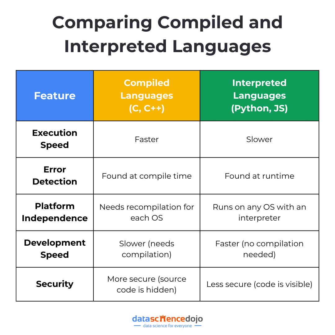
Compiled vs. Interpreted Languages: How Java and Python Execute Code?
Ever wondered why Java applications tend to run faster than Python scripts? Or why Python lets you test code instantly without compiling? It all comes down to how these languages are executed.
Programming languages generally fall into two categories – compiled and interpreted. This distinction affects everything from performance and debugging to how easily your code runs across different systems. Let’s break it down!
What is a Compiled Language?
A compiled language takes your entire code and converts it into machine code (binary) before running the program. This process is handled by a compiler, which generates an independent executable file (like .exe or .class).
Once compiled, the program can run directly on the computer’s hardware without needing the original source code. Think of it like translating a book where, instead of translating each page as you read, you translate the whole thing first, so you can read it smoothly later. This ensures:
- Faster execution – Since the code is pre-compiled, the program runs much more efficiently
- Optimized performance – The compiler fine-tunes the code before execution, making better use of system resources
- Less flexibility for quick edits – Any changes require a full recompilation, which can slow down development
Common examples of compiled languages include C, C++, and Java. These languages prioritize speed and efficiency, making them ideal for performance-intensive applications.
What is an Interpreted Language?
Unlike compiled languages that translate code all at once, interpreted languages work in real time, executing line by line as the program runs. Instead of a compiler, they rely on an interpreter, which reads and processes each instruction on the fly.
Think of it like a live translator at an international conference where, instead of translating an entire speech beforehand, the interpreter delivers each sentence as it is spoken. This offers:
- Instant execution – No need to compile; just write your code and run it immediately
- Easier debugging – If something breaks, the interpreter stops at that line, making it simpler to track errors
- Slower performance – Since the code is being processed line by line, it runs slower compared to compiled programs
It includes examples like Python, JavaScript, PHP, and Ruby. These languages are all about convenience and quick iteration, making them perfect for developers who want to write, test, and modify code on the go.

How Java and Python Handle Execution?
Now that we know the difference between compiled and interpreted languages, let’s see where Java and Python fit in.
Java: A Hybrid Approach
Java takes a middle-ground approach that is not fully compiled like C++, nor fully interpreted like Python. Instead, it follows a two-step execution process:
- Compiles to Bytecode – Java code is first converted into an intermediate form called bytecode
- Runs on the Java Virtual Machine (JVM) – The bytecode is not executed directly by the computer but runs on the JVM, making Java platform-independent
To boost performance, Java also uses Just-In-Time (JIT) compilation, which converts bytecode into native machine code at runtime, improving speed without losing flexibility.
Python: Fully Interpreted
Python, on the other hand, sticks to a purely interpreted approach. Key steps of Python execution include:
- Compiling to Bytecode: Java code is first compiled into an intermediate form called bytecode (.class files)
- Running on the JVM: This bytecode is not executed directly by the system but runs on the Java Virtual Machine (JVM), making Java platform-independent
- JIT Compilation for Speed: Java uses Just-In-Time (JIT) compilation, which converts bytecode into native machine code at runtime, optimizing performance
- Python Interpreter: It reads and executes code line by line, skipping the need for compilation
This makes Python slower in execution compared to Java, but much faster for development and debugging, since you do not need to compile every change.
Explore the NLP techniques and tasks to implement using Python
While understanding how Java and Python execute code gives us a solid foundation, there is more to this debate than just compilation vs. interpretation. These two languages have key differences that shape how developers use them. Let’s dive deeper into the major differences between Java and Python and see which one fits your needs best!
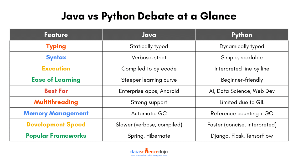
Java vs Python: Key Differences Every Developer Should Know
Now that we’ve explored how Java and Python execute code, let’s dive into the key differences that set them apart. Whether you’re choosing a language for your next project or just curious about how they compare, understanding these aspects will help you make an informed decision.

1. Syntax & Readability
One of the biggest differences between Java and Python is their syntax. Let’s understand this difference with an example of printing “Hello, World!” in both languages.
Python is known for its clean, simple, and English-like syntax. It focuses on readability, reducing the need for extra symbols like semicolons or curly braces. As a result, Python code is often shorter and easier to write, making it a great choice for beginners.
You can print “Hello, World!” in Python using the following code:
Java, on the other hand, is more structured and verbose. It follows a strict syntax that requires explicit declarations, semicolons, and curly braces. While this adds some complexity, it also enforces consistency, which is beneficial for large-scale applications.
In Java, the same output can be printed using the code below:
As you can see, Python gets straight to the point, while Java requires more structure.
2. Speed & Performance
Performance is another key factor when comparing Java vs Python.
Java is generally faster because it uses Just-In-Time (JIT) compilation, which compiles bytecode into native machine code at runtime, improving execution speed. Java is often used for high-performance applications like enterprise software, banking systems, and Android apps.
Python is slower since it executes code line by line. However, performance can be improved with optimized implementations like PyPy or by using external libraries written in C (e.g., NumPy for numerical computations). Python is still fast enough for most applications, especially in AI, data science, and web development.
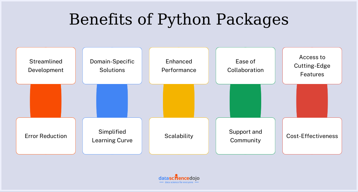
Here’s a list of top Python packages you must explore
3. Typing System (Static vs. Dynamic)
Both programming languages also differ in ways they handle data types. This difference can be highlighted in the way a variable is declared in both languages.
Java is statically typed – You must declare variable types before using them. This helps catch errors early and makes the code more predictable, but requires extra effort when coding. This static typing makes it more reliable, helps prevent errors, but requires more code. For instance:
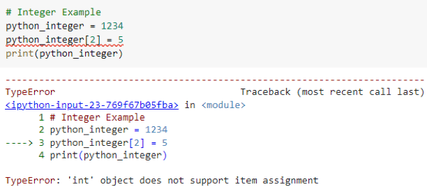
Python is dynamically typed – Variables do not require explicit type declarations, making development faster. While this can lead to unexpected errors at runtime, it also makes the language faster to write and more flexible. Such a variable declaration in Python will look like:
4. Memory Management & Garbage Collection
Both Java and Python automatically manage memory, but they do it differently. Let’s take a closer look at how each programming language gets it done.
Java uses automatic garbage collection via the Java Virtual Machine (JVM), which efficiently handles memory allocation and cleanup. Its garbage collector runs in the background, optimizing performance without manual intervention. Hence, it is more optimized to handle large-scale applications.
Python also has garbage collection, but it mainly relies on reference counting. When an object’s reference count drops to zero, it is removed from memory. However, Python’s memory management can sometimes lead to inefficiencies, especially in large applications.
5. Concurrency & Multithreading
Similarly, when it comes to multithreading and parallel execution, both Java and Python handle it differently.
Java excels in multithreading. Thanks to its built-in support for threads, Java allows true parallel execution, making it ideal for applications requiring high-performance processing, like gaming engines or financial software.
Python, on the other hand, faces limitations due to the Global Interpreter Lock (GIL). The GIL prevents multiple threads from executing Python bytecode simultaneously, which limits true parallelism. However, it supports multiprocessing, helping bypass the GIL for CPU-intensive tasks.
You can also learn to build a recommendation system using Python
Thus, when it comes to Java vs Python, there is no one-size-fits-all answer. If you need speed, performance, and scalability, Java is the way to go. If you prioritize simplicity, rapid development, and flexibility, Python is your best bet.
Java vs Python: Which One to Use for Your Next Project?
Now that we’ve explored the key differences between Java and Python, the next big question is: Which one should you use for your next project?
To answer this question, you must understand where each of these language excel. While both languages have carved out their own niches in the tech world, let’s break it down further for better understanding.
Where to Use Java?
Java’s reliability, speed, and scalability make it a top choice for several critical applications. A few key ones are discussed below:
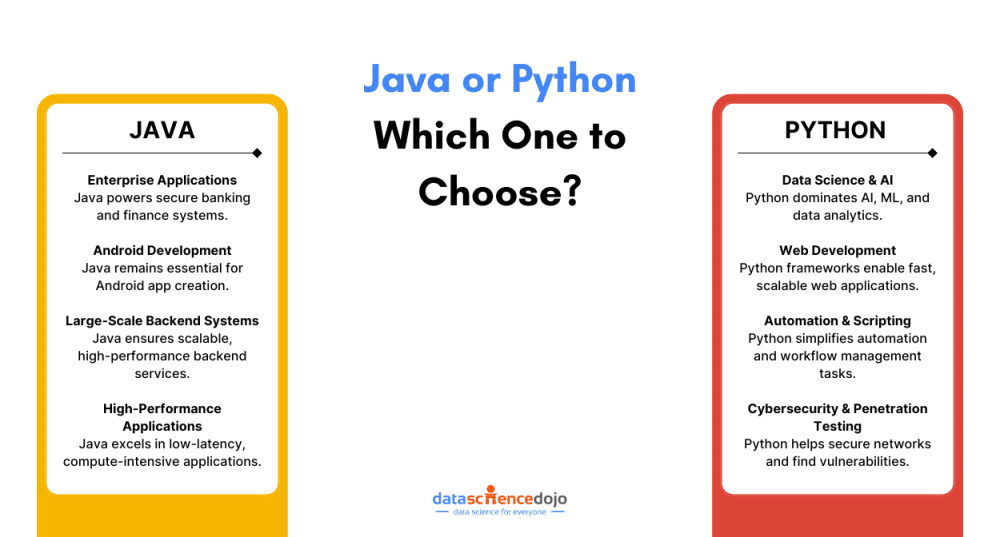
- Enterprise Applications (Banking, Finance, and More)
Java has long been the backbone of banking and financial applications, as they need secure, fast, and highly scalable systems. Many large enterprises rely on Java frameworks like Spring and Hibernate to build and maintain their financial software. For instance, global banks like Citibank and JPMorgan Chase use Java for their core banking applications.
- Android Development
While Kotlin has gained traction in recent years, Java is still widely used for Android app development. Since Android apps run on the Dalvik Virtual Machine (DVM), which is similar to the Java Virtual Machine (JVM), Java remains a go-to language for Android developers. Popular Android apps built using Java include Spotify and Twitter.
- Large-Scale Backend Systems
Java’s robust ecosystem makes it ideal for handling complex backend systems. Frameworks like Spring Boot and Hibernate help developers build secure, scalable, and high-performance backend services. Even today, E-commerce giants like Amazon and eBay rely on Java for their backend operations.
- High-Performance Applications
Java is a compiled language with Just-In-Time (JIT) compilation, performing better in compute-intensive applications compared to interpreted languages like Python. This makes it ideal for applications that require fast execution, low latency, and high reliability, like stock trading platforms and high-frequency trading (HFT) systems.
When to Choose Python?
Meanwhile, Python’s flexibility, simplicity, and powerful libraries make it the preferred choice for data-driven applications, web development, and automation. Let’s look closer at the preferred use cases for the programming language.
- Data Science, AI, and Machine Learning
Python has become the best choice for AI and machine learning. With libraries like TensorFlow, PyTorch, NumPy, and Pandas, Python makes it incredibly easy to develop and deploy data science and AI models. Google, Netflix, and Tesla use Python for AI-driven recommendations, data analytics, and self-driving car software.
Learn to build AI-based chatbots using Python
- Web Development (Django, Flask)
Python’s simplicity and rapid development capabilities make it suitable for web development. Frameworks like Django and Flask allow developers to build secure, scalable web applications quickly. For instance, websites like Instagram and Pinterest are built using Python and Django.
- Automation and Scripting
Automation is one of the strengths of Python, making it a top choice for data scraping, server management, or workflow automation. Python can save hours of manual work with just a few lines of code. Its common use is in companies like Reddit and NASA for automating tasks like data analysis and infrastructure management.
- Cybersecurity and Penetration Testing
Python is widely used in ethical hacking and cybersecurity due to its ability to automate security testing, develop scripts for vulnerability scanning, and perform network penetration testing. Security professionals use Python to identify system weaknesses and secure networks. Popular security tools like Metasploit and Scapy are built using Python.
You can also learn about Python in data science.

To sum it up:
- Java for large-scale enterprise applications, Android development, or performance-heavy systems
- Python for AI, data science, web development, or automation
And if you still cannot make up your mind, you can always learn both languages!

Java or Python? Making the Right Choice for Your Future
Both languages are in high demand, with Python leading in AI and automation and Java dominating enterprise and backend systems. No matter which one you choose, you’ll be investing in a skill that opens doors to exciting career opportunities in the ever-evolving tech world.
The best language for you depends on where you want to take your career. Since both are the best choices in their domains, whether you choose Python’s flexibility or Java’s robustness, you will be setting yourself up for a thriving tech career!