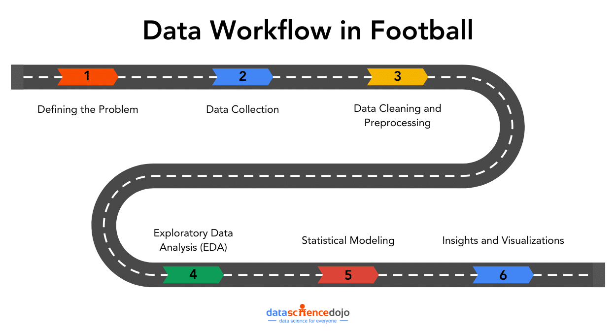
In the world of data, data workflows are essential to providing the ideal insights. Similarly, in football, these workflows will help you gain a competitive edge and optimize team performance.
Imagine you’re the data analyst for a top football club, and after reviewing the performance from the start of the season, you spot a key challenge: the team is creating plenty of chances, but the number of goals does not reflect those opportunities.
The coaching team is now counting on you to find a data-driven solution. This is where a data workflow is essential, allowing you to turn your raw data into actionable insights.
In this article, we’ll explore how that workflow – covering aspects from data collection to data visualizations – can tackle the real-world challenges. Whether you’re passionate about football or data, this journey highlights how smart analytics can increase performance.
1. Defining the Problem
The starting point for any successful data workflow is problem definition. For a football data analyst, this involves turning the team’s goals or challenges into specific, measurable questions that can be analyzed with data.
Problem
The football team you work for has struggled in front of the goal lately. With one of the lowest goal tallies in the league, this has seen them slip down into the bottom half of the table.
Using this problem, your question might become:“How can we increase our shot conversion rate to score more goals?”
Techniques
Stakeholder Meetings: Scheduling regular meetings with coaches, scouts, and analysts might help you pinpoint the problem. Coaches might identify that players are not taking high-percentage shots, while analysts can frame this into a data-driven question.
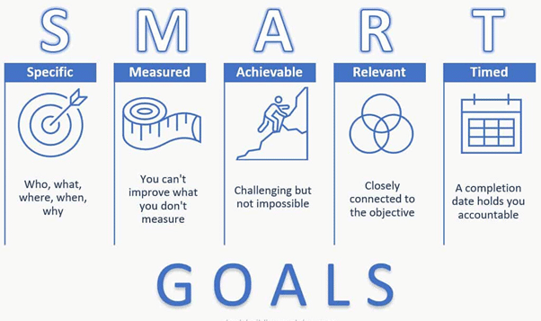
SMART: Using the SMART (Specific, Measurable, Achievable, Relevant, and Time-Bound) framework, you can provide a clear and measurable goal. For instance, “Increase shot conversion rate by 10% over the next 5 matches”.
A well-defined question helps focus data collection and analysis on solving a tangible issue that can be measured and tracked.
2. Data Collection
Once the problem is defined, the next step in the data workflow is collecting relevant data. In football analytics, this could mean pulling data from several sources, including event and player performance data.
Types of Football Data
Event Data: Shot locations, types (on-target/off-target), and outcomes (goal or miss).
Tracking Data: Player movements and positioning.
Player Metrics: Shot accuracy, shot attempts, and other similar metrics.
Techniques
Data Integration: Often, you might need to pull data from multiple sources and combine these datasets. Providers like Opta, Statsbomb, and Wyscout provide users with data from different leagues all over the world. FBRef provides users with football statistics for free, while Statsbomb offers a few free resources for event data for practice. In Power BI, you can merge these sources through data transformation, while in Python, libraries like pandas are used to integrate and join different datasets.
Real-Time Data Collection: Football teams increasingly use real-time tracking and wearable technologies to capture live player data during matches, which can be analyzed post-game for immediate insights.
You may combine event data (e.g., shot types and results) with tracking data (e.g., player positioning) to see where players are when they take the shot, allowing you to assess the quality of the shooting opportunity.
Effective data collection ensures you have all the necessary information to begin the analysis, setting the stage for reliable insights into improving shot conversion rates or any other defined problem.
3. Data Cleaning and Preprocessing
After collecting data, the next critical step in the data workflow is data cleaning. Typically, datasets can have errors, missing values, or inconsistencies, so ensuring your data is clean and well-structured is essential for accurate analysis.
Before diving into cleaning, it’s important to first understand the data’s structure and quality through data profiling. Data profiling helps identify issues such as missing values, duplicates, or outliers.
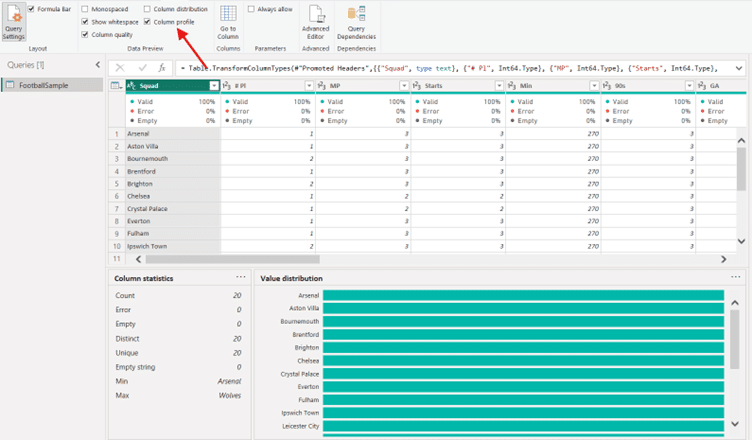
In Power BI: You can use the ‘Column Profile’ option to quickly view data completeness, data types, and patterns, helping you detect any inconsistencies early.
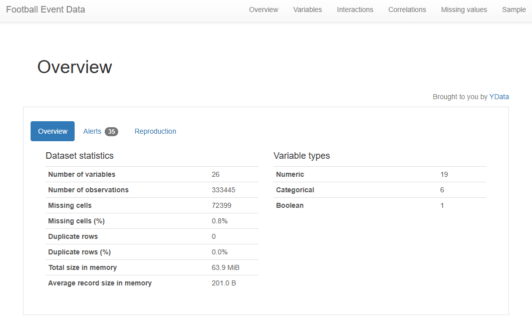
In Python: Data profiling, such as pandas-profiling (now renamed to ydata-profiling), generate reports that highlight potential problems, giving you a detailed overview of the dataset.
Key Data Cleaning Techniques
Handling Missing Data:
Imputation: Estimate missing values using the mean or median.
Removal: Exclude rows or columns with excessive missing values.
Data Normalization:
Normalize metrics to per 90 to fairly compare players with different playing times.
You might come across certain matches that have missing data on shot outcomes, or any other metric. Correcting these issues ensures your analysis is based on clean, reliable data.
4. Exploratory Data Analysis (EDA)
With clean data in hand, the next step is Exploratory Data Analysis (EDA). This phase is crucial for uncovering trends and relationships that will help explain why the team’s shot conversion rate is low.
Techniques for EDA
Descriptive Statistics: Start by calculating average shot distance, conversion rates, and shot success inside vs. outside the penalty area.
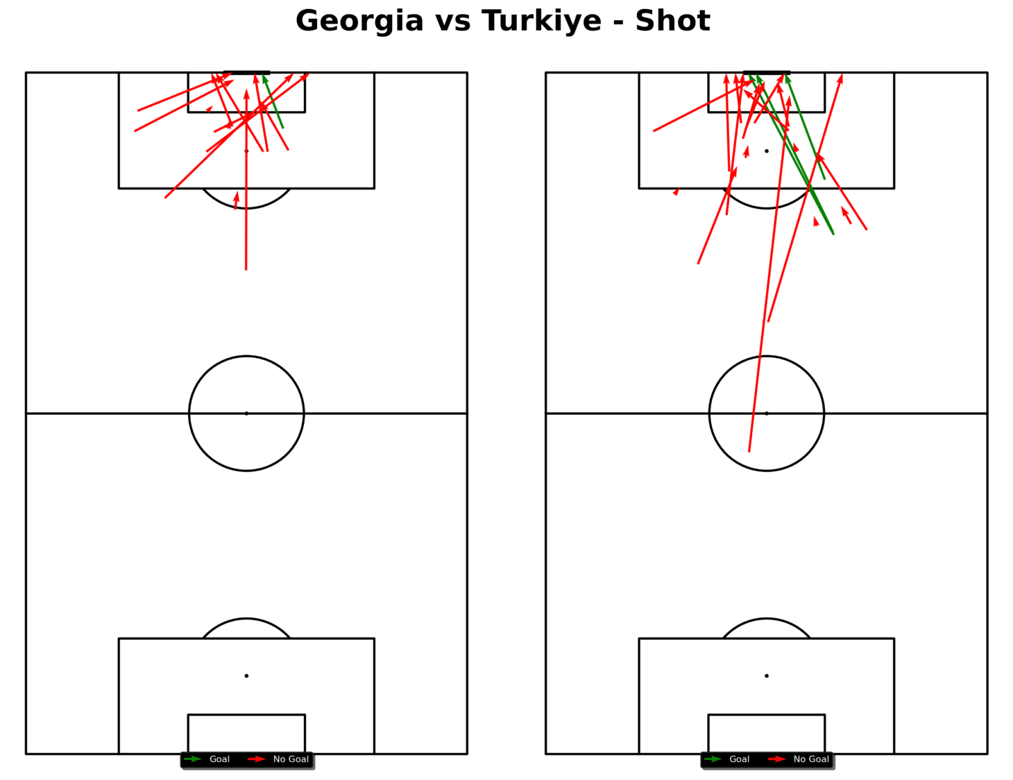
Data Visualization: Create shot maps using Python or Power BI to visualize where shots are taken and their success rates.
Shot map from Georgia vs Turkiye (Euros 2024)
A simple way to plot a shot map, like the one above, would be as follows:
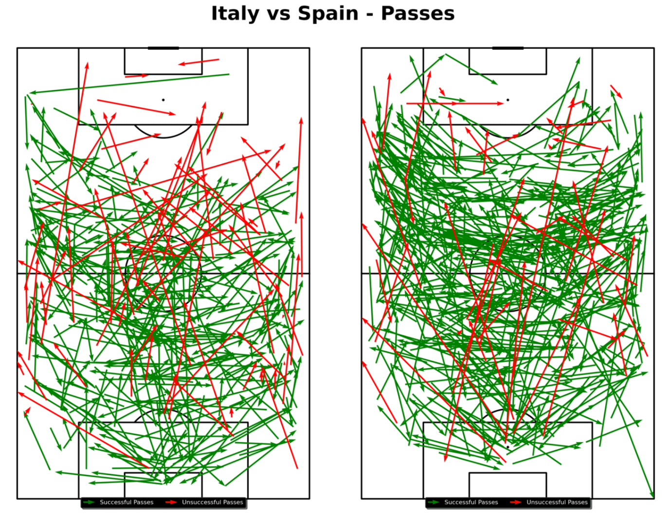
Passing Networks and Maps:Analyze passing networks and pass maps to see the build-up to shots and goals.
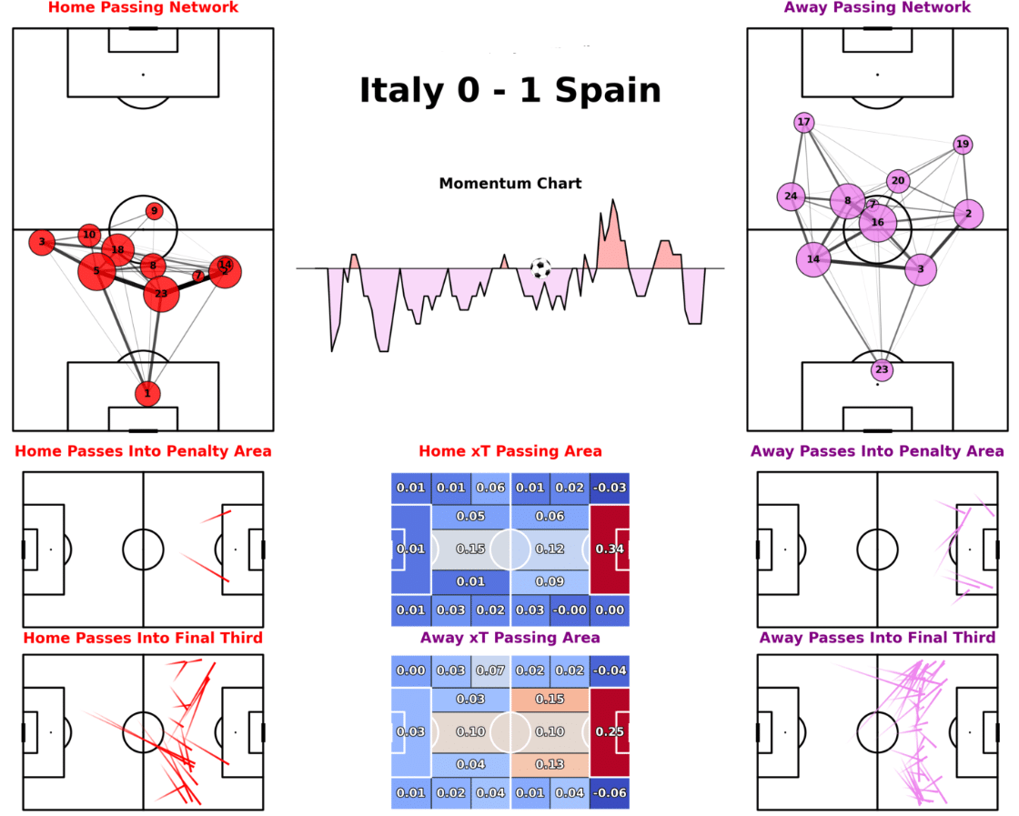
Pass map for Italy vs Spain (Euros 2024)
For this specific pass map, which shows both teams from a certain game, you could utilize the following Python code:
Visualizations created in Python or Power BI might show that most shots are coming from low-percentage areas, such as outside the penalty box. This visualization suggests that to improve shot conversion, the team should focus on creating chances in higher-percentage areas inside the box.
EDA provides key insights into trends that directly affect the team’s shot conversion rate, allowing you to identify specific areas for improvement.
Do not be afraid to dive deep and explore other techniques. This is the part where analysts should embrace their curiosity and learn new approaches along the way.
5. Statistical Modelling
Statistical modelling can provide deeper insights into football data, though it’s not always necessary. Different types of models can help analyze different aspects and predict outcomes.
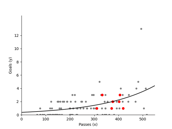
Poisson Regression: Useful for predicting the number of goals a team is likely to score based on shot attempts, passes, and other factors.
Predicting Goals Based on Passes
Below you’ll find a lesson fromDr. David Sumpter, a professor and author, who dives deep into statistical models and their application in football.
While statistical models aren’t required for every analysis, they can offer a tactical edge by providing detailed predictions and insights that inform decision-making.
6. Insights and Visualizations
Once the data has been analyzed, the final step is telling the story. Football coaches and management may not be familiar with technical data terms, so presenting the data clearly is crucial.
Football Insights Techniques
Power BI Dashboards: Power BI dashboards provide an intuitive way to present key insights like shot maps, player metrics, and overall conversion rates. Coaches can use these dashboards to monitor performance in real time and adjust strategies accordingly.
Static Reports: Making a static report could be another option. Reports can provide you with a comprehensive view of data and are suitable for in-depth analysis. To make reports, you could combine visualizations made in Power BI or Python and display them in a PowerPoint presentation or a document assembled in Canva.
Example from a Match Report with Simple Visualizations
So, from this example match report, you can understand how a certain team might have played or dominated throughout this game. For instance, the momentum chart is heavily favouring Spain which means they dominated throughout the game. Furthermore, the passing networks show which side the teams favoured more and how they were set up to play.
For visualizations like the one above, you can access the GitHub repository from which this code was referenced here.
Clear communication of data-driven insights allows teams to act on the analysis, completing the data workflow and directly impacting performance on the pitch.
A structured data workflow is essential for modern football teams looking to improve their performance. By following each phase – from problem definition to data cleaning, analysis, and visualization – teams can turn raw data into actionable insights that directly enhance on-field outcomes.
Hello there, dear reader! It’s an absolute pleasure to have you here. Today, we’re embarking on a thrilling journey into the heart of data-driven marketing. Don’t worry, though; this isn’t your average marketing chat!
We’re delving into the very science that makes marketing tick. So, grab a cup of tea, sit back, and let’s unravel the fascinating ties between marketing Trust me, it’s going to be a real hoot!
The art and science of marketing
Isn’t it remarkable how marketing has evolved over the years? We’ve moved from straightforward newspaper adverts and radio jingles to a more complex, intricate world of digital marketing. It’s not just about catchy slogans and vibrant posters anymore.
No, no, marketing now is a careful blend of creativity, psychology, technology, and – you’ve guessed it: science. Marketing, you see, isn’t just an art; it’s a science. It involves careful experimentation, research, and above all, analysis.
Understanding data-driven marketing in 2023
We’re in a world brimming with data, and marketers are akin to modern-day alchemists. They skilfully transmute raw, overwhelming data into golden insights, driving powerful marketing strategies.
And that, dear friends, is what we’re delving into today – the captivating world of data analysis in marketing. Exciting, isn’t it? Let’s forge ahead!
The role of data analysis in marketing
Data, dear reader, is the unsung hero of our digital age. It’s everywhere, and it’s valuable. In marketing, it’s like a crystal ball that shows trends, customer behaviors, campaign performance, and more. The trick, though, lies in making sense of this raw data, and that’s where data analysis sweeps in.
Data analysis in marketing is like decoding a treasure map. It involves scrutinizing information to identify patterns, trends, and insights.
These insights then guide decision-making, inform strategies, and help evaluate the success of campaigns.
And it’s not just about retrospective analysis; predictive analytics can forecast future trends, helping businesses stay one step ahead. Quite incredible, wouldn’t you say?
Understanding your audience: The heart of effective marketing
No matter how innovative or creative your marketing strategies are, they’ll fall flat without a deep understanding of your audience. And guess what? Data analysis is the key to unlocking this understanding.
Data analysis helps peel back the layers of your audience’s behaviours, preferences, and needs. It’s like having a conversation with your customers without them saying a word. You learn what makes them tick, what they love, and what they don’t.
This level of understanding enables businesses to create highly targeted marketing campaigns that resonate with their audience. It’s all about delivering the right message, to the right people, at the right time. And it’s data analysis that helps nail this trifecta.
The impact of data-driven marketing
The magic of data-driven marketing lies in its power to deliver measurable, tangible results. It’s not just about casting a wide net and hoping for the best. Instead, it’s about making informed decisions based on real, credible data.
When done right, data-driven marketing can skyrocket brand visibility, foster customer loyalty, and drive business growth. It’s a bit like having a secret weapon in the competitive business landscape. And who wouldn’t want that?
Exciting future of data-driven marketing
If you think data-driven marketing is impressive now, just wait until you see what the future holds! We’re looking at advanced artificial intelligence (AI) models, predictive analytics, and machine learning algorithms that can dive even deeper into data, delivering unprecedented insights.
The future of marketing is not just reactive but proactive, not just personalized but hyper-personalized. It’s about predicting customer needs even before they arise, delivering a marketing experience that’s truly tailored and unique.
Exciting times lie ahead, dear reader, and data analysis will be at the heart of it all. So, as we embrace this data-driven era, it’s essential to appreciate the remarkable science that underpins successful marketing.
After all, data analysis isn’t just a cog in the marketing machine; it’s the engine that drives it. And that, friends, is the power and promise of data-driven marketing.
Diving deeper into data analysis
So, you’re still with us? Fantastic! Now that we’ve skimmed the surface, it’s time to dive deeper into the wonderful ocean of data analysis. Let’s break down the types of data your business can leverage and the techniques to analyse them. Ready? Onwards we go!
Types of data in marketing
Data is like the language your customers use to speak to you, and there are different ‘dialects you need to be fluent in. Here are the primary types of data used in marketing:
Demographic data: This type of data includes basic information about your customers such as age, gender, location, income, and occupation. It helps businesses understand who their customers are.
Psychographic data: This is a step deeper. It involves understanding your customers’ attitudes, interests, lifestyles, and values. It paints a picture of why your customers behave the way they do.
Behavioral data: This includes purchasing behaviors, product usage, and interactions with your brand. It gives you a peek into what your customers do.
Feedback data: This comes directly from your customers via reviews, surveys, and social media. It shows how your customers perceive your brand.
All these types of data, when analyzed and understood, provide rich, nuanced insights about your customer base. It’s like assembling a jigsaw puzzle where every piece of data adds more detail to the picture.
Techniques in data analysis
Now, let’s get our hands a little dirty and dig into some common techniques used in data analysis:
Descriptive Analysis: This involves understanding past trends and behaviors. It answers the question, “What happened?”
Diagnostic Analysis: This dives deeper into why something happened. It’s like a post-mortem that helps identify the causes of a particular outcome.
Predictive Analysis: As the name suggests, this technique is all about forecasting future trends and behaviors based on past data.
Prescriptive Analysis: This is the most advanced form of data analysis. It suggests courses of action to take for future outcomes.
Using these techniques, marketers can transform raw data into actionable insights. It’s quite similar to a cook turning raw ingredients into a delicious meal!
Data analysis tools: The magic wand for marketers
In our data-driven world, numerous tools help marketers analyze and interpret data. These tools are like magic wands, transforming data into visually appealing and easily understandable formats.
Google Analytics: It provides insights into website traffic, user behaviors, and the performance of online marketing campaigns.
Tableau: It’s a visual analytics platform that transforms raw data into interactive, real-time dashboards.
Looker: It’s a business intelligence tool that delivers detailed insights about customer behaviors and business performance.
HubSpot: This is an all-in-one marketing tool that offers customer relationship management, social media management, content marketing, and, of course, data analytics.
These tools empower marketers to not only collect data but also interpret it, visualize it, and share insights across their teams.
The Power of A/B Testing
Now, here’s something particularly exciting! Have you ever found yourself torn between two options, unable to decide which is better? Well, in marketing, there’s a fantastic way to make that decision – A/B testing!
A/B testing, also known as split testing, is a method to compare two versions of a web page, email, or other marketing asset to see which performs better. It’s a practical, straightforward way to test changes to your marketing campaigns before implementing them.
For instance, if you’re not sure whether a green or a red button will drive more clicks on your website, simply test both versions. The one that garners more clicks wins! It’s that simple, and it’s all thanks to the science of data analysis.
Bringing it all together
So, there you have it! We’ve taken a whirlwind tour through the fascinating world of data-driven marketing. But, as they say, the proof of the pudding is in the eating.
So, it’s time for businesses to roll up their sleeves and embrace data analysis in their marketing. It’s time to unlock the powerful potential of data-driven marketing.
Remember, in our digital age, data isn’t just a byproduct; it’s a vital strategic asset. So, here’s to harnessing the power of data analysis for more effective, efficient, and successful marketing campaigns. Cheers!
Heatmaps are a type of data visualization that uses color to represent data values. For the unversed,
data visualization is the process of representing data in a visual format. This can be done through charts, graphs, maps, and other visual representations.
What are heatmaps?
A heatmap is a graphical representation of data in which values are represented as colors on a two-dimensional plane. Typically, heatmaps are used to visualize data in a way that makes it easy to identify patterns and trends.
Heatmaps are often used in fields such as data analysis, biology, and finance. In data analysis, heatmaps are used to visualize patterns in large datasets, such as website traffic or user behavior.
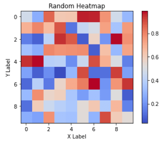
In biology, heatmaps are used to visualize gene expression data or protein-protein interaction networks. In finance, heatmaps are used to visualize stock market trends and performance.This diagram shows a random 10×10 heatmap using `NumPy` and `Matplotlib`.
Heatmaps
Advantages of heatmaps
Visual representation: Heatmaps provide an easily understandable visual representation of data, enabling quick interpretation of patterns and trends through color-coded values.
Large data visualization: They excel at visualizing large datasets, simplifying complex information and facilitating analysis.
Comparative analysis: They allow for easy comparison of different data sets, highlighting differences and similarities between, for example, website traffic across pages or time periods.
Customizability: They can be tailored to emphasize specific values or ranges, enabling focused examination of critical information.
User-friendly: They are intuitive and accessible, making them valuable across various fields, from scientific research to business analytics.
Interactivity: Interactive features like zooming, hover-over details, and data filtering enhance the usability of heatmaps.
Effective communication: They offer a concise and clear means of presenting complex information, enabling effective communication of insights to stakeholders.
Creating heatmaps using “Matplotlib”
We can create heatmaps using Matplotlib by following the aforementioned steps:
To begin, we import the necessary libraries, namely Matplotlib and NumPy.
Following that, we define our data as a 3×3 NumPy array.
Afterward, we utilize Matplotlib’s imshow function to create a heatmap, specifying the color map as ‘coolwarm’.
To enhance the visualization, we incorporate a color bar by employing Matplotlib’s colorbar function.
Subsequently, we set the title and axis labels using Matplotlib’s set_title, set_xlabel, and set_ylabel functions.
Lastly, we display the plot using the show function.
Bottom line: This will create a simple 3×3 heatmap with a color bar, title, and axis labels.
Customizations available in Matplotlib for heatmaps
Following is a list of the customizations available for Heatmaps in Matplotlib:
Changing the color map
Changing the axis labels
Changing the title
Adding a color bar
Adjusting the size and aspect ratio
Setting the minimum and maximum values
Adding annotations
Adjusting the cell size
Masking certain cells
Adding borders
These are just a few examples of the many customizations that can be done in heatmaps using Matplotlib. Now, let’s see all the customizations being implemented in a single example code snippet:
In this example, the heatmap is customized in the following ways:
Set the colormap to ‘coolwarm’
Set the minimum and maximum values of the colormap using `vmin` and `vmax`
Set the size of the figure using `figsize`
Set the extent of the heatmap using `extent`
Set the linewidth of the heatmap using `linewidth`
Add a colorbar to the figure using the `colorbar`
Set the title, xlabel, and ylabel using `set_title`, `set_xlabel`, and `set_ylabel`, respectively
Add annotations to the heatmap using `text`
Mask certain cells in the heatmap by setting their values to `np.nan`
Show the frame around the heatmap using `set_frame_on(True)`
First, we import the necessary libraries: seaborn, matplotlib, and numpy.
Next, we generate a random 10×10 matrix of numbers using NumPy’s rand function and store it in the variable data.
We create a heatmap by using Seaborn’s heatmap function. It takes the data as input and specifies the color map using the cmap parameter. Additionally, we set the annot parameter to True to display the values in each cell of the heatmap.
To enhance the plot, we add a title, x-label, and y-label using Matplotlib’s title, xlabel, and ylabel functions.
Finally, we display the plot using the show function from Matplotlib.
Overall, the code generates a random heatmap using Seaborn with a color map, annotations, and labels using Matplotlib.
Customizations available in Seaborn for heatmaps:
Following is a list of the customizations available for Heatmaps in Seaborn:
Change the color map
Add annotations to the heatmap cells
Adjust the size of the heatmap
Display the actual numerical values of the data in each cell of the heatmap
Add a color bar to the side of the heatmap
Change the font size of the heatmap
Adjust the spacing between cells
Customize the x-axis and y-axis labels
Rotate the x-axis and y-axis tick labels
Now, let’s see all the customizations being implemented in a single example code snippet:
In this example, the heatmap is customized in the following ways:
Set the color palette to “Blues”.
Add annotations with a font size of 10.
Set the x and y labels and adjust font size.
Set the title of the heatmap.
Adjust the figure size.
Show the heatmap plot.
Limitations of heatmaps:
Heatmaps are a useful visualization tool for exploring and analyzing data, but they do have some limitations that you should be aware of:
Limited to two-dimensional data: They are designed to visualize two-dimensional data, which means that they are not suitable for visualizing higher-dimensional data.
Limited to continuous data: They are best suited for continuous data, such as numerical values, as they rely on a color scale to convey the information. Categorical or binary data may not be as effectively visualized using heatmaps.
May be affected by color blindness: Some people are color blind, which means that they may have difficulty distinguishing between certain colors. This can make it difficult for them to interpret the information in a heatmap.
Can be sensitive to scaling: The color mapping in a heatmap is sensitive to the scale of the data being visualized. Therefore, it is important to carefully choose the color scale and to consider normalizing or standardizing the data to ensure that the heatmap accurately represents the underlying data.
Can be misleading: They can be visually appealing and highlight patterns in the data, but they can also be misleading if not carefully designed. For example, choosing a poor color scale or omitting important data points can distort the visual representation of the data.
It is important to consider these limitations when deciding whether or not to use a heatmap for visualizing your data.
Conclusion
Heatmaps are powerful tools for visualizing data patterns and trends. They find applications in various fields, enabling easy interpretation and analysis of large datasets. Matplotlib and Seaborn offer flexible options to create and customize heatmaps. However, it’s essential to understand their limitations, such as two-dimensional data representation and sensitivity to color perception. By considering these factors, heatmaps can be a valuable asset in gaining insights and communicating information effectively.
The finance industry has traditionally been driven by human expertise and intuition. However, with the explosion of data and the advent of new technologies, the industry is starting to embrace the use of artificial intelligence (AI) to manage and analyze this data. This has led to the emergence of the financial technology (FinTech) industry, which is focused on using technology to make financial services more accessible, efficient, and customer friendly.
AI in FinTech is like having a financial expert who never sleeps, never gets tired, and never complains about coffee.
AI has been at the forefront of this transformation, helping companies to automate repetitive tasks, make more informed decisions, and improve customer experience. In FinTech, AI has been particularly valuable, given the massive amounts of data that financial institutions generate. AI-powered algorithms can process this data, identify trends and patterns, and help companies to better understand their customers and offer personalized financial products and services.
Continue reading to know more about artificial intelligence (AI) in the financial technology (FinTech) industry, and how it is transforming the finance industry.
Exploring the Popularity of AI: An Overview
AI is changing the way we work, live, and handle money. It’s making things faster, smarter, and more efficient across different industries—but one of the biggest areas seeing its impact is finance.
In banking and financial services, AI helps detect fraud, manage risks, and automate customer support with chatbots. It can analyze huge amounts of data in seconds, helping banks make smarter lending decisions and offering customers personalized investment advice. If you’ve ever used a budgeting app that tracks your spending or gotten a quick loan approval online, AI was likely behind it.
Beyond banking, AI is transforming stock trading, helping investors make better decisions with predictive analytics. It’s also improving security, flagging suspicious transactions in real-time to prevent fraud. Even insurance companies use AI to assess claims faster and offer better pricing.
AI isn’t just making financial services more efficient—it’s also making them more accessible. More people can now get loans, investment advice, and secure banking services, no matter where they are. As AI keeps evolving, it’s set to make finance smarter, safer, and more personalized than ever.
A Bird’s-Eye View: AI and FinTech
The FinTech industry is built on innovation and disruption. It has always been focused on using technology to make financial services more accessible, efficient, and customer friendly. AI is at the forefront of this innovation, helping companies to take their services to the next level.
One of the most significant benefits of AI in FinTech is that it allows companies to make more informed decisions. AI-powered algorithms can process vast amounts of data and identify trends and patterns that would be impossible for humans to detect. This allows financial institutions to make more accurate predictions and improve their risk management strategies.
Another benefit of AI in FinTech is the ability to automate repetitive tasks. Many financial institutions still rely on manual processes, which are time-consuming and prone to errors. AI-powered systems can automate these tasks, freeing up employees to focus on more complex and value-adding activities.
AI is also making a big impact on customer experience. AI-powered chatbots and virtual assistants can provide customers with 24/7 support and personalized recommendations, improving customer satisfaction and loyalty. AI can also help financial institutions to better understand their customers’ needs and preferences, enabling them to offer tailored financial products and services.
Exploring Opportunities: How AI Is Revolutionizing the FinTech Future
The use of AI in the FinTech industry also presents significant opportunities for financial institutions to improve their operations and better serve their customers. Here are some of the key opportunities:
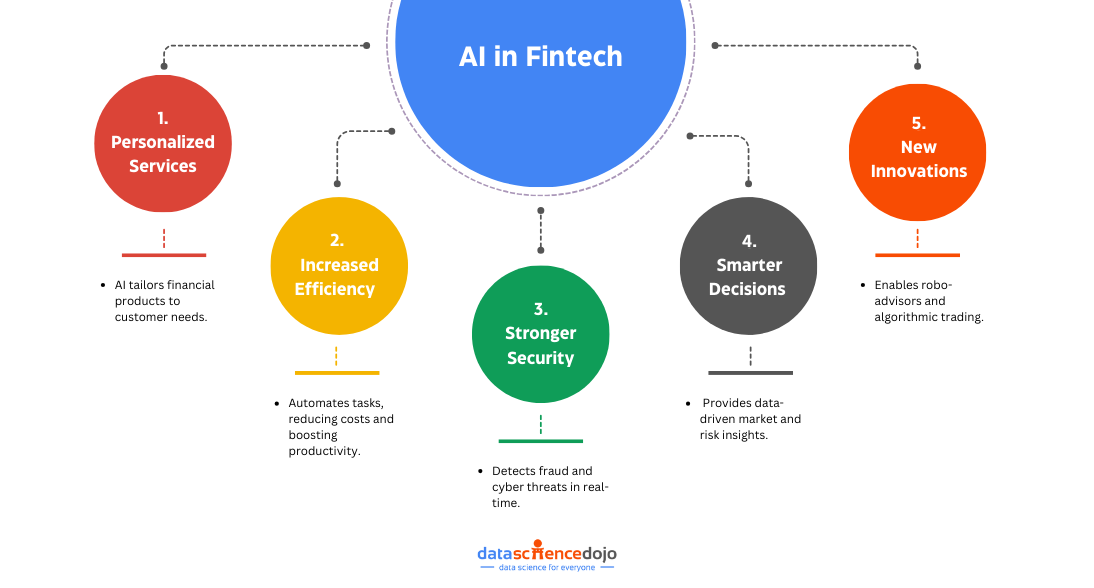
1. Improved Customer Experience
AI-powered systems can help financial institutions better understand their customers and their needs. By using AI to analyze customer data, companies can provide personalized services and tailored financial products that better meet the needs of individual customers.
2. Enhanced Efficiency
AI can automate repetitive and time-consuming tasks, such as data entry and fraud detection, freeing up employees to focus on more complex and value-adding activities. This can lead to increased productivity, reduced costs, and faster response times.
3. Better Risk Management
AI can help financial institutions to identify and mitigate potential risks, such as fraud and cyber threats. By analyzing large amounts of data, AI can detect unusual patterns and suspicious activities, enabling companies to take proactive measures to prevent or minimize risk.
4. Enhanced Decision-Making
AI-powered systems can provide financial institutions with more accurate and timely insights, enabling them to make more informed decisions. By using AI to analyze data from multiple sources, companies can gain a better understanding of market trends, customer preferences, and potential risks.
5. New Business Opportunities
AI can enable financial institutions to develop new products and services, such as robo-advisors and algorithmic trading. These innovations can help companies to expand their offerings and reach new customer segments.
Future Trends in AI and FinTech
As AI continues to evolve, its role in FinTech is expanding, paving the way for smarter, more efficient, and accessible financial services. Several key trends are shaping the future of AI in FinTech, driving innovation and transforming how financial institutions operate.
AI-Powered Wealth Management
AI is redefining wealth management by offering intelligent, data-driven insights for investors. Robo-advisors, powered by AI, are becoming more sophisticated, providing personalized investment strategies based on real-time market analysis and individual risk tolerance.
These tools enable investors—both seasoned professionals and newcomers—to make informed decisions with minimal effort. Machine learning models can also predict market trends, helping financial firms optimize portfolio management and mitigate risks.
Green FinTech and Sustainable Finance
Sustainability is becoming a major focus in finance, and AI is playing a crucial role in promoting green FinTech solutions. AI-driven algorithms help assess ESG (Environmental, Social, and Governance) criteria, allowing investors to make responsible investment choices.
FinTech firms are using AI to develop carbon footprint tracking tools, enabling businesses and individuals to monitor and reduce their environmental impact. Additionally, AI is improving efficiency in green lending by assessing the sustainability of projects and optimizing funding allocation for environmentally friendly initiatives.
Integration of Central Bank Digital Currencies (CBDCs)
With central banks worldwide exploring the potential of digital currencies, AI is expected to play a significant role in their implementation. AI-driven analytics can enhance the security and efficiency of CBDC transactions, ensuring smooth integration with existing financial systems.
Moreover, AI-powered fraud detection can help monitor and prevent illicit activities within digital currency networks. As CBDCs gain traction, AI will be instrumental in managing risks, improving transaction speeds, and ensuring regulatory compliance.
Navigating Challenges of AI in FinTech
Using AI in the FinTech industry presents several challenges that need to be addressed to ensure the responsible use of this technology. Two of the primary challenges are fairness and bias, and data privacy and security.
The first challenge relates to ensuring that the algorithms used in AI are fair and unbiased. These algorithms are only as good as the data they are trained on, and if that data is biased, the algorithms will be too. This can result in discrimination and unfair treatment of certain groups of people. The FinTech industry must address this challenge by developing AI algorithms that are not only accurate but also fair and unbiased, and regularly auditing these algorithms to address any potential biases.
The second challenge is data privacy and security. Financial institutions handle sensitive personal and financial data, which must be protected from cyber threats and breaches. While AI can help identify and mitigate these risks, it also poses new security challenges. For instance, AI systems can be vulnerable to attacks that manipulate or corrupt data. The FinTech industry must implement robust security protocols and ensure that AI systems are regularly audited for potential vulnerabilities. Additionally, they must comply with data privacy regulations to safeguard customer data from unauthorized access or misuse.
Conclusion
Through AI in FinTech, financial institutions can manage and analyze their data more effectively, improve efficiency and accuracy, and provide better financial services to customers. While there are challenges associated with using AI in FinTech, the opportunities are vast, and the potential benefits are enormous. As the finance industry continues to evolve, AI will be a game-changer in managing the finance of the future.
Python has become the backbone of data science, offering powerful tools for data analysis, visualization, and machine learning. If you want to harness the power of Python to kickstart your data science journey, Data Science Dojo’s “Introduction to Python for Data Science” course is the perfect starting point.
This course equips you with essential Python skills, enabling you to manipulate data, build insightful visualizations, and apply machine learning techniques. In this blog, we’ll explore how this course can help you unlock the full power of Python and elevate your data science expertise.
Why Learn Python for Data Science?
Python has become the go-to language for data science, thanks to its simplicity, flexibility, and vast ecosystem of open-source libraries. The power of Python for data science lies in its ability to handle data analysis, visualization, and machine learning with ease.
Its easy-to-learn syntax makes it accessible to beginners, while its powerful tools cater to advanced data scientists. With a large community of developers constantly improving its capabilities, Python continues to dominate the data science landscape.
One of Python’s biggest advantages is that it is an interpreted language, meaning you can write and execute code instantly—no need for a compiler. This speeds up experimentation and makes debugging more efficient.
Applications Showcasing the Power of Python for Data Science
1. Data Analysis Made Easy
Python simplifies data analysis by providing libraries like pandas and NumPy, which allow users to clean, manipulate, and process data efficiently. Whether you’re working with databases, CSV files, or APIs, the power of Python for data science enables you to extract insights from raw data effortlessly.
2. Stunning Data Visualizations
Data visualization is essential for making sense of complex datasets, and Python offers several powerful libraries for this purpose. Matplotlib, Seaborn, and Plotly help create interactive and visually appealing charts, graphs, and dashboards, reinforcing the power of Python for data science in storytelling.
3. Powering Machine Learning
Python is a top choice for machine learning, with libraries like scikit-learn, TensorFlow, and PyTorch making it easy to build and train predictive models. Whether it’s image recognition, recommendation systems, or natural language processing, the power of Python for data science makes AI-driven solutions accessible.
4. Web Scraping for Data Collection
Need to gather data from websites? Python makes web scraping simple with libraries like BeautifulSoup, Scrapy, and Selenium. Businesses and researchers leverage the power of Python for data science to extract valuable information from the web for market analysis, sentiment tracking, and competitive research.
Why Choose Data Science Dojo for Learning Python?
With so many Python courses available, choosing the right one can be overwhelming. Data Science Dojo’s “Introduction to Python for Data Science” stands out as a top choice for both beginners and professionals looking to build a strong foundation in Python for data science. Here’s why this course is worth your time and investment:
1. Hands-On, Instructor-Led Training
Unlike self-paced courses that leave you figuring things out on your own, this course offers live, instructor-led training that ensures you get real-time guidance and support. With expert instructors, you’ll learn best practices and gain industry insights that go beyond just coding.
2. Comprehensive Curriculum Covering Essential Data Science Skills
The course is designed to take you from Python basics to real-world data science applications. You’ll learn: ✔ Python fundamentals – syntax, variables, data structures ✔ Data wrangling – cleaning and preparing data for analysis ✔ Data visualization – using Matplotlib and Seaborn for insights ✔ Machine learning – an introduction to predictive modeling
3. Practical Learning with Real-World Examples
Theory alone isn’t enough to master Python for data science. This course provides hands-on exercises, coding demos, and real-world datasets to ensure you can apply what you learn in actual projects.
4. 12 + Months of Learning Platform Access
Even after the live sessions end, you won’t be left behind. The course grants you more than twelve months of access to its learning platform, allowing you to revisit materials, practice coding, and solidify your understanding at your own pace.
5. Earn CEUs and Boost Your Career
Upon completing the course, you receive over 2 Continuing Education Units (CEUs), an excellent addition to your professional credentials. Whether you’re looking to transition into data science or enhance your current role, this certification can give you an edge in the job market.
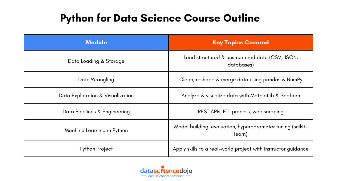
Python for Data Science Course Outline
Data Science Dojo’s “Introduction to Python for Data Science” course provides a structured, hands-on approach to learning Python, covering everything from data handling to machine learning. Here’s what you’ll learn:
1. Data Loading, Storage, and File Formats
Understanding how to work with data is the first step in any data science project. You’ll learn how to load structured and unstructured data from various file formats, including CSV, JSON, and databases, making data easily accessible for analysis.
2. Data Wrangling: Cleaning, Transforming, Merging, and Reshaping
Raw data is rarely perfect. This module teaches you how to clean, reshape, and merge datasets, ensuring your data is structured and ready for analysis. You’ll master data transformation techniques using Python libraries like pandas and NumPy.
3. Data Exploration and Visualization
Data visualization helps in uncovering trends and insights. You’ll explore techniques for analyzing and visualizing data using popular Python libraries like Matplotlib and Seaborn, turning raw numbers into meaningful graphs and reports.
4. Data Pipelines and Data Engineering
Data engineering is crucial for handling large-scale data. This module covers: ✔ RESTful architecture & HTTP protocols for API-based data retrieval ✔ The ETL (Extract, Transform, Load) process for data pipelines ✔ Web scraping to extract real-world data from websites
5. Machine Learning in Python
Learn the fundamentals of machine learning with scikit-learn, including: ✔ Building and evaluating models ✔ Hyperparameter tuning for improved performance ✔ Working with different estimators for predictive modeling
6. Python Project – Apply Your Skills
The course concludes with a hands-on Python project where you apply everything you’ve learned. With instructor guidance, you’ll work on a real-world project, helping you build confidence and gain practical experience.
Frequently Asked Questions
How long do I have access to the program content? Access to the course content depends on the plan you choose at registration. Each plan offers different durations and levels of access, so be sure to check the plan details to find the one that best fits your needs.
What is the duration of the program? The Introduction to Python for Data Science program spans 5 days with 3 hours of live instruction each day, totaling 15 hours of training. There’s also additional practice available if you want to continue refining your Python skills after the live sessions.
Are there any prerequisites for this program? No prior experience is required. However, our pre-course preparation includes tutorials on fundamental data science concepts and Python programming to help you get ready for the training.
Are classes taught live or are they self-paced? Classes are live and instructor-led. In addition to the interactive sessions, you’ll have access to office hours for additional support. While the program isn’t self-paced, homework assignments and practical exercises are provided to reinforce your learning, and lectures are recorded for later review.
What is the cost of the program? The program cost varies based on the plan you select and any discounts available at the time. For the most up-to-date pricing and information on payment plans, please contact us at [email protected]
What if I have questions during the live sessions or while working on homework? Our sessions are highly interactive—students are encouraged to ask questions during class. Instructors provide thorough responses, and a dedicated Discord community is available to help you with any questions during homework or outside of class hours.
What different plans are available? We offer three plans:
Dojo: Includes 15 hours of live training, pre-training materials, course content, and restricted access to Jupyter notebooks.
Guru: Includes everything in the Dojo plan plus bonus Jupyter notebooks, full access to the learning platform during the program, a collaboration forum, recorded sessions, and a verified certificate from the University of New Mexico worth 2 Continuing Education Credits.
Sensei: Includes everything in the Guru plan, along with one year of access to the learning platform, Jupyter notebooks, collaboration forums, recorded sessions, office hours, and live support throughout the program.
Are there any discounts available? Yes, we are offering an early-bird discount on all three plans. Check the course page for the latest discount details.
How much time should I expect to spend on class and homework? Each class is 3 hours per day, and you should plan for an additional 1–2 hours of homework each night. Our instructors and teaching assistants are available during office hours from Monday to Thursday for extra help.
How do I register for the program? To register, simply review the available packages on our website and sign up for the upcoming cohort. Payments can be made online, via invoice, or through a wire transfer.
Explore the Power of Python for Data Science
The power of Python for data science makes it the top choice for data professionals. Its simplicity, vast libraries, and versatility enable efficient data analysis, visualization, and machine learning.
Mastering Python can open doors to exciting opportunities in data-driven careers. A structured course, like the one from Data Science Dojo, ensures hands-on learning and real-world application.
Start your Python journey today and take your data science skills to the next level
Data analysis is an essential process in today’s world of business and science. It involves extracting insights from large sets of data to make informed decisions. One of the most common ways to represent a data analysis is through code. However, is code the best way to represent a data analysis?
In this blog post, we will explore the pros and cons of using code to represent data analysis and examine alternative methods of representation.
Advantages of performing data analysis through code
One of the main advantages of representing data analysis through code is the ability to automate the process. Code can be written once and then run multiple times, saving time and effort. This is particularly useful when dealing with large sets of data that need to be analyzed repeatedly.
Additionally, code can be easily shared and reused by other analysts, making collaboration and replication of results much easier.Another advantage of code is the ability to customize and fine-tune the analysis. With it, analysts have the flexibility to adjust the analysis as needed to fit specific requirements. This allows for more accurate and tailored results.
Furthermore, code is a powerful tool for data visualization, enabling analysts to create interactive and dynamic visualizations that can be easily shared and understood.
Disadvantages of performing data analysis through code
One of the main disadvantages of representing data analysis through code is that it can be challenging for non-technical individuals to understand. It is often written in specific programming languages, which can be difficult for non-technical individuals to read and interpret. This can make it difficult for stakeholders to understand the results of the analysis and make informed decisions.
Another disadvantage of code is that it can be time-consuming and requires a certain level of expertise. Analysts need to have a good understanding of programming languages and techniques to be able to write and execute code effectively. This can be a barrier for some individuals, making it difficult for them to participate in the entire process.
Code represents data analysis
Alternative methods of representing data analysis
1. Visualizations
One alternative method of representing data analysis is through visualizations. Visualizations, such as charts and graphs, can be easily understood by non-technical individuals and can help to communicate complex ideas in a simple and clear way. Additionally, there are tools available that allow analysts to create visualizations without needing to write any code, making it more accessible to a wider range of individuals.
2. Natural language
Another alternative method is natural language. Natural Language Generation (NLG) software can be used to automatically generate written explanations of analysis in plain language. This makes it easier for non-technical individuals to understand the results and can be used to create reports and presentations.
Narrative: Instead of representing data through code or visualizations, a narrative format can be used to tell a story about the data. This could include writing a report or article that describes the findings and conclusions of the analysis.
Dashboards: Creating interactive dashboards allows users to easily explore the data and understand the key findings. Dashboards can include a combination of visualizations, tables, and narrative text to present the data in a clear and actionable way.
Machine learning models: Using machine learning models to analyze data can also be an effective way to represent the data analysis. These models can be used to make predictions or identify patterns in the data that would be difficult to uncover through traditional techniques.
Presentation: Preparing a presentation for the data analysis is also an effective way to communicate the key findings, insights, and conclusions effectively. This can include slides, videos, or other visual aids to help explain the data and the analysis.
Ultimately, the best way to represent data analysis will depend on the audience, the data, and the goals of the analysis. By considering multiple methods and choosing the one that best fits the situation, it can be effectively communicated and understood.
Code is a powerful tool for representing data analysis and has several advantages, such as automation, customization, and visualization capabilities. However, it also has its disadvantages, such as being challenging for non-technical individuals to understand and requiring a certain level of expertise.
Alternative methods, such as visualizations and natural language, can be used to make data analysis more accessible and understandable for a wider range of individuals. Ultimately, the best way to represent a data analysis will depend on the specific context and audience.
An overview of data analysis, the data analysis methods, its process, and implications for modern corporations.
Studies show that 73% of corporate executives believe that companies failing to use data analysis on big data lack long-term sustainability. While data analysis can guide enterprises to make smart decisions, it can also be useful for individual decision-making.
Let’s consider an example of using data analysis at an intuitive individual level. As consumers, we are always choosing between products offered by multiple companies. These decisions, in turn, are guided by individual past experiences. Every individual analysis the data obtained via their experience to generate a final decision.
Put more concretely, data analysis involves sifting through data, modeling it, and transforming it to yield information that guides strategic decision-making. For businesses, data analytics can provide highly impactful decisions with long-term yield.
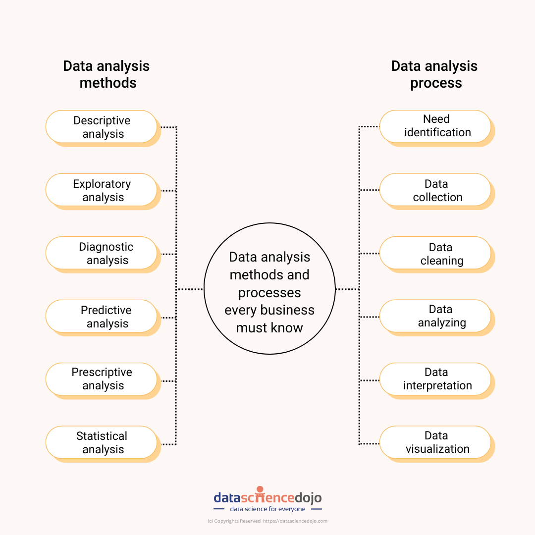
Data analysis methods and data analysis processes – Data Science Dojo
So, let’s dive deep and look at how data analytics tools can help businesses make smarter decisions.
The data analysis process
The process includes five key steps:
1. Identify the need
Companies use data analytics for strategic decision-making regarding a specific issue. The first step, therefore, is to identify the particular problem. For example, a company decides it wants to reduce its production costs while maintaining product quality. To do so effectively, the company would need to identify step(s) of the workflow pipeline it should implement cost cuts.
Similarly, the company might also have a hypothetical solution to its question. Data analytics can be used to judge the falsifiability of the hypothesis, allowing the decision-maker to reach the optimized solution.
A specific question or hypothesis determines the subsequent steps of the process. Hence, this must be as clear and specific as possible.
2. Collect the data
Once the data analysis need is identified, the subsequent kind of data is also determined. Data collection can involve data entered in different types and formats. One broad classification is based on structure and includes structured and unstructured data.
Structured data, for example, is the data a company obtains from its users via internal data acquisition methods such as marketing automation tools. More importantly, it follows the usual row-column database and is suited to the company’s exact needs.
Unstructured data, on the other hand, need not follow any such formatting. It is obtained via third parties such as Google Trends, census bureaus, world health bureaus, and so on. Structured data is easier to work with as it’s already tailored to the company’s needs. However, unstructured data can provide a significantly larger data volume.
There are many other data types to consider as well. For example, metadata, big data, real-time data, and machine data.
3. Clean the data
The third step, data cleaning, ensures that error-free data is used for the data analysis. This step includes procedures such as formatting data correctly and consistently, removing any duplicate or anomalous entries, dealing with missing data, and fixing cross-set data errors.
Performing these tasks manually is tedious and hence, various tools exist to smoothen the data-cleaning process. These include open-source data tools such as OpenRefine, desktop applications like Trifacta Wrangler, cloud-based software as a service (SaaS) like TIBCO Clarity, and other data management tools such as IBM Infosphere quality stage especially used for big data.
4. Perform data analysis
Data analysis includes several methods as described earlier. The method to be implemented depends closely on the research question to be investigated. Data analysis methods are discussed in detail later in this blog.
5. Present the results
Presentation of results defines how well the results are to be communicated. Visualization tools such as charts, images, and graphs effectively convey findings, establishing visual connections in the viewer’s mind. These tools emphasize patterns discovered in existing data and shed light on predicted patterns, assisting the results’ interpretation.
Listen to the Data Analysis challenges in cybersecurity
Data analysis methods
Data analysts use a variety of approaches, methods, and tools to deal with data. Let’s sift through these methods from an approach-based perspective:
1. Descriptive analysis
Descriptive analysis involves categorizing and presenting broader datasets in a way that allows emergent patterns to be observed from them to see if there are any obvious patterns. Data aggregation techniques are one way of performing descriptive analysis. This involves first collecting the data and then sorting it to ease manageability.
This can also involve performing statistical analysis on the data to determine, say, the measures of frequency, dispersion, and central tendencies that provide a mathematical description for the data.
2. Exploratory analysis
Exploratory analysis involves consulting various data sets to see how certain variables may be related, or how certain patterns may be driving others. This analytic approach is crucial in framing potential hypotheses and research questions that can be investigated using data analytic techniques.
Data mining, for example, requires data analysts to use exploratory analysis to sift through big data and generate hypotheses to be tested.
3. Diagnostic analysis
Diagnostic analysis is used to answer why a particular pattern exists in the first place. For example, this kind of analysis can assist a company in understanding why its product is performing in a certain way in the market.
Diagnostic analytics includes methods such as hypothesis testing, determining correlations v/s causation, and diagnostic regression analysis.
4. Predictive analysis
Predictive analysis answers the question of what will happen. This type of analysis is key for companies in deciding new features or updates on existing products, and in determining what products will perform well in the market.
For predictive analysis, data analysts use existing results from the earlier described analyses while also using results from machine learning and artificial intelligence to determine precise predictions for future performance.
5. Prescriptive analysis
Prescriptive analysis involves determining the most effective strategy for implementing the decision arrived at. For example, an organization can use prescriptive analysis to sift through the best way to unroll a new feature. This component of data analytics actively deals with the consumer end, requiring one to work with marketing, human resources, and so on.
Prescriptive analysis makes use of machine learning algorithms to analyze large amounts of big data for business intelligence. These algorithms can assess large amounts of data by working through them via “if” and “else” statements and making recommendations accordingly.
6. Quantitative and qualitative analysis
Quantitative analysis computationally implements algorithms testing out a mathematical fit to describe correlation or causation observed within datasets. This includes regression analysis, null analysis, hypothesis analysis, etc.
Qualitative analysis, on the other hand, involves non-numerical data such as interviews and pertains to answering broader social questions. It involves working closely with textual data to derive explanations.
7. Statistical analysis
Statistical techniques provide answers to essential decision challenges. For example, they can accurately quantify risk probabilities, predict product performance, establish relationships between variables, and so on. These techniques are used by both qualitative and quantitative analysis methods. Some of the invaluable statistical techniques for data analysts include linear regression, classification, resampling methods, and subset selection.
Statistical analysis, more importantly, lies at the heart of data analysis, providing the essential mathematical framework via which analysis is conducted.
Data-driven businesses
Data-driven businesses use the data analysis methods described above. As a result, they offer many advantages and are particularly suited to modern needs. Their credibility relies on them being evidence-based and using precise mathematical models to determine decisions.
Some of these advantages include stronger customer needs, precise identification of business needs, devising effective strategy decisions, and performing well in a competitive market. Data-driven businesses are the way forward.
Data analysis and data science are very closely related professions in many respects. If one enjoys problem-solving, data-driven decision-making, and critical thinking, both occupations are a good fit.
While all alternatives draw on the same core skill set and strive toward comparable goals, there are differences in schooling, talents, daily responsibilities, and compensation ranges. In this blog, we will explore the data analyst vs data scientist debate in detail.
The data science certification course offers insight into the tools, technology, and trends driving the data science revolution. We have developed this guide to enable you to go through the abilities and background required to become a data scientist or data analyst, and their corresponding course fee.
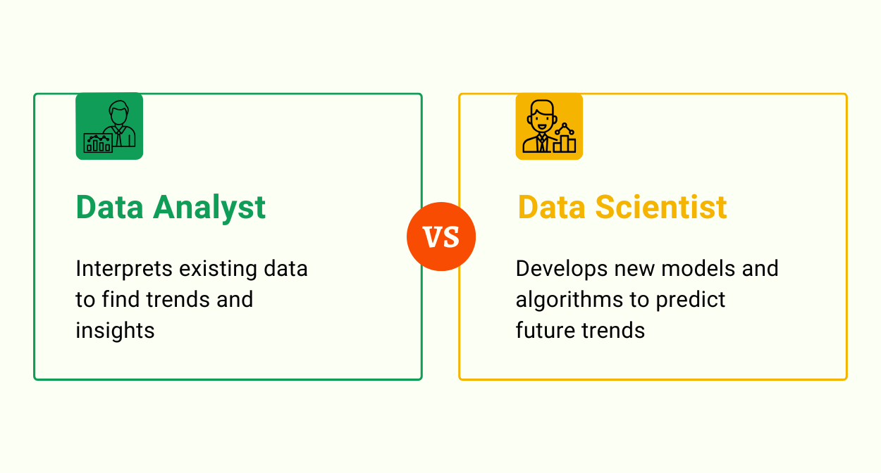
Data Analyst vs Data Scientist
Data analysis and data science are often misunderstood since they rely on the same fundamental skills, not to mention the very same broad educational foundation (e.g., advanced mathematics, and statistical analysis).
However, the day-to-day responsibilities of each role are vastly different. The difference, in its most basic form, is how they utilize the data they collect.
Key differences between a data analyst and a data scientist
Role of a Data Analyst
A data analyst examines gathered information, organizes it, and cleans it to make it clear and helpful. Based on the data acquired, they make recommendations and judgments. They are part of a team that converts raw data into knowledge that can assist organizations in making sound choices and investments.
Role of a Data Scientist
A data scientist creates the tools that will be used by an analyst. They write programs, algorithms, and data-gathering technologies. Data scientists are innovative problem solvers who are constantly thinking of new methods to acquire, store, and view data.
Differences in the Role of Data Scientist and Data Analyst
Job roles of data analyst and data scientist
While both data analysts and data scientists deal with data, the primary distinction is what they do with it. Data analysts evaluate big data sets for insights, generate infographics, and generate visualizations to assist corporations in making better strategic choices. Data scientists, on the other hand, use models, methods, predictive analytics, and specialized analyses to create and build current innovations for data modeling and manufacturing.
Data experts and data scientists typically have comparable academic qualifications. Most have Bachelor’s degrees in economics, statistics, computer programming, or machine intelligence. They have in-depth knowledge of data, marketing, communication, and algorithms. They can work with advanced systems, databases, and Programming environments.
What is Data Analysis?
Data analysis is the thorough examination of data to uncover trends that can be turned into meaningful information. When formatted and analyzed correctly, previously meaningless data can become a wealth of useful and valuable information that firms in various industries can use.
Data analysis, for example, can tell a technical store what product is most successful at what period and with which population, which can then help employees decide what kind of incentives to run. Data analysis may also assist social media companies in determining when, what, and how they should promote particular users to optimize clicks.
What is Data Science?
Data science and data analysis both aim to unearth significant insights within piles of complicated or seemingly minor information. Rather than performing the actual analytics, data science frequently aims at developing the models and implementing the techniques that will be used during the process of data analysis.
While data analysis seeks to reveal insights from previous data to influence future actions, data science seeks to anticipate the result of future decisions. Artificial image processing and pattern recognition, which are still in their early stages, are used to create predictions based on large amounts of historical data.
Responsibilities: Data Scientist vs Data Analyst
Professionals in data science and data analysis must be familiar with managing data, information systems, statistics, and data analysis. They must alter and organize data for relevant stakeholders to find it useful and comprehensible.
They also assess how effectively firms perform on predefined metrics, uncover trends, and explain the differentiated strategy. While job responsibilities frequently overlap, there are contrasts between data scientists and data analysts, and the methods they utilize to attain these goals.
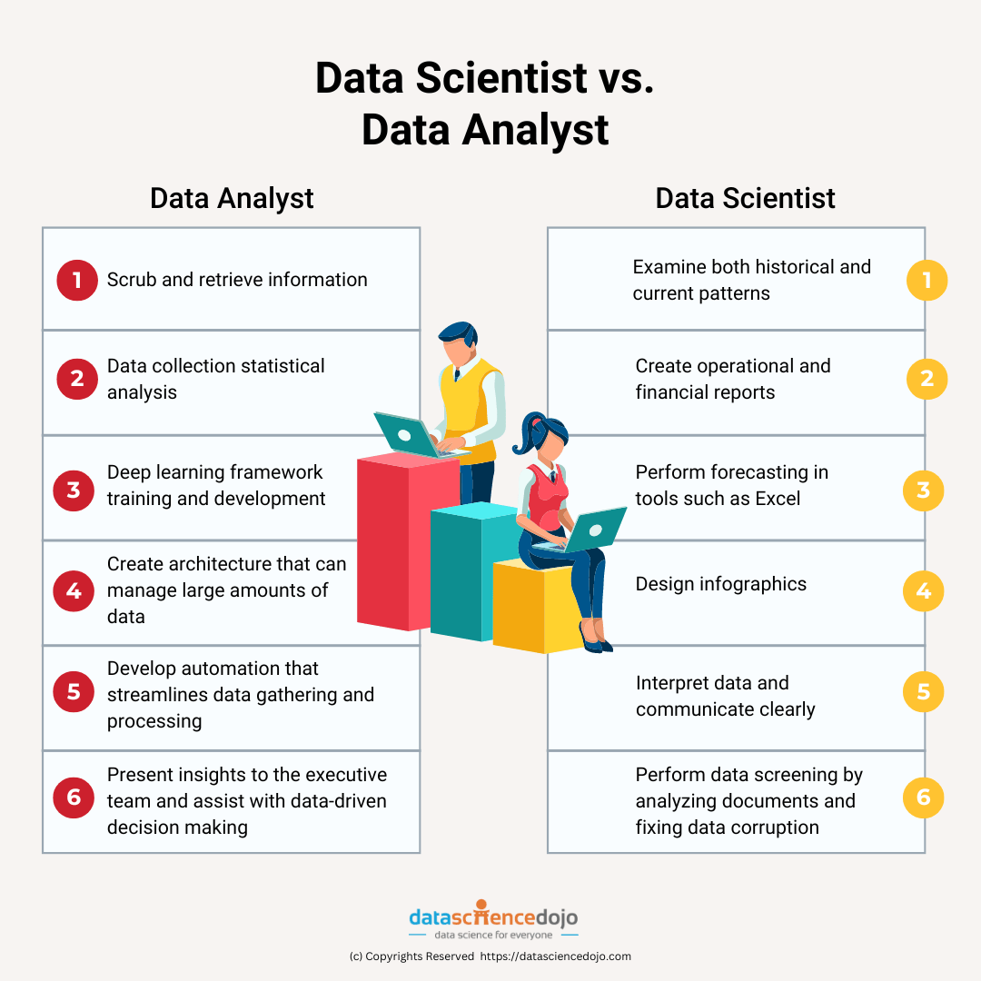
Data Analyst
Data Scientist
Data analyzers are expert interpreters. They use massive amounts of information to comprehend what is going on in the industry and how corporate actions affect how customers perceive and engage with the company. They are motivated by the need to understand people’s perspectives and behaviors through data analysis.
Data scientists build the framework for capturing data and better understanding the narrative it conveys about the industry, enterprise, and decisions taken. They are designers that can create a system that can handle the volume of data required while also making it valuable for understanding patterns and advising the management team.
Everyday data analyst tasks may involve examining both historical and current patterns and trends.
Data scientists are typically responsible for the scrubbing and information retrieval.
Create operational and financial reports.
Data collection statistical analysis.
Forecasting in tools such as Excel.
Deep learning framework training and development.
Designing infographics.
Creating architecture that can manage large amounts of data.
Data interpretation and clear communication.
Developing automation that streamlines data gathering and processing chores daily.
Data screening is accomplished by analyzing documents and fixing data corruption.
Presenting insights to the executive team and assisting with data-driven decision making
Using predictive modeling to discover and impact future trends.
Role: Data Scientist vs Data Analyst
Data Analyst Job Description
A data analyst, unsurprisingly, analyzes data. This entails gathering information from various sources and processing it via data manipulation and statistical techniques. These procedures organize and extract insights from data, which are subsequently given to individuals who may act on them.
Become a pro with Data Analytics with these 12 amazing books
Users and decision-makers frequently ask data analysts to discover answers to their inquiries. This entails gathering and comparing pertinent facts and stitching them together to form a larger picture. Knowledgehut looks more closely at a career path in analytics and science, and helps you determine which employment best matches your interests, experience, and ambitions.
Data Scientist Job Description
A data scientist can have various tasks inside a corporation, among which are very comparable to those of a data analyst, such as gathering, processing, and analyzing data to get meaningful information.
Whereas a data analyst is likely to have been given particular questions to answer, a data scientist may indeed evaluate the same collection of data with the goal of diverse variables that may lead to a new line of inquiry. In other words, a data scientist must identify both the appropriate questions and the proper answers.
A data scientist will make designs and write algorithms and software to assist them as well as their research analyst team members with the analysis of data. A data scientist is also deeply engaged in the field of artificial intelligence and tries to push the limits and develop new methods to apply this technology in a corporate context.
How can Data Scientists become Ethical Hackers?
Yes, you heard it right. Data scientists can definitely become ethical hackers. There are several skills data scientists possess that can help them with the smooth transition from data scientists to ethical hackers. The skills are extensive knowledge of programming languages, databases, and operating systems. Data science is an important tool that can prevent hacking.
The necessary skills for a data scientist to become an ethical hacker include mathematical and statistical expertise, and extensive hacking skills. With the rise of cybercrimes, the need for cyber security is increasing. When data scientists become ethical hackers, they can protect an organization’s data and prevent cyber-attacks.
Skill Set Required for Data Analysis and Data Science
Data Analysis
Data Science
Qualification: A Bachelor’s or Master’s degree in a related discipline, such as mathematics or statistics.
Qualification: An advanced degree, such as a master’s degree or possibly a Ph.D., in a relevant discipline, such as statistics, computer science, or mathematics.
Language skills: To understand data analysis, such as Python, SQL, CQL, and R.
Language skills: Demonstrate proficiency in data-related programming languages such as SQL, R, Java, and Python.
Soft skills:
Written and verbal communication skills
Exceptional analytical skills
Organizational skills
The ability to manage many products at the same time may be required.
Soft skills:
Substantial experience with data mining
Specialized statistical activities and tools
Generating generalized linear model regressions, statistical tests, designing data structures, and text mining.
Technical skills:
Expertise in data gathering and some of the most recent data analytics technology.
Technical skills:
Experience with data sources and web services
Web services such as Spark, Hadoop, DigitalOcean and S3
Trained to use information obtained from third-party suppliers such as Google Analytic, Crimson Hexagon, Coremetrics, Site Catalyst
Microsoft Office proficiency:
Proficient in Microsoft Office applications, notably Excel, to properly explain their findings and translate them for others to grasp.
Knowledge of statistical techniques and technology: Data processing technologies such as MySQL and Gurobi, as well as technological advances such as machine learning models, deep learning, artificial intelligence, artificial neural networks, and decision tree learning, will play a significant role.
Conclusion
Each career is a good fit for an individual who enjoys statistics, analytics, and evaluating business decisions. As a data analyst or data scientist, you will make logical sense of large amounts of data, articulate patterns and trends, and participate in great responsibilities in a corporate or government organization.
When picking between data analytics and a data science profession, evaluate your career aspirations, skills, and how much time you want to devote to higher learning and intensive training. Start your data analyst or data scientist journey with a data science course with a nominal data science course fee to learn in-demand skills used in realistic, long-term projects, strengthening your resume and commercial viability.
FAQs
Which is better: Data science or data analysis?
Data science is suitable for candidates who want to develop advanced machine-learning models and make human tasks easier. On the other hand, the data analyst role is appropriate for candidates who want to begin their career in data analysis.
What is the career path for data analytics and data science?
Most data analysts will begin their careers as junior members of a bigger data analysis team, where they will learn the fundamentals of the work in a hands-on environment and gain valuable experience in data manipulation. At the senior level, data analysts become team leaders, in control of project selection and allocation.
A junior data scientist will most likely obtain a post with a focus on data manipulation before delving into the depths of learning algorithms and mapping out forecasts. The procedure of preparing data for analysis varies so much from case to case that it’s far simpler to learn by doing.
Once conversant with the mechanics of data analysis, data scientists might expand their understanding of artificial intelligence and its applications by designing algorithms and tools. A more experienced data scientist may pursue team lead or management positions, distributing projects and collaborating closely with users and decision-makers.
Alternatively, they could use their seniority to tackle the most difficult and valuable problems using their specialist expertise in patterns and machine learning.
What is the salary for a data scientist and a data analyst in India?
2 to 4 years (Senior Data Analyst): $98,682 whereas the average data scientist salary is $100,560, according to the U.S. Bureau of Labor Statistics.
To perform a systematic study of data, we use data science life cycle to perform testable methods to make predictions.
Before you apply science to data, you must be aware of the important steps. A data science life cycle will help you get a clear understanding of the end-to-end actions of a data scientist. It provides us with a framework to fulfill business requirements using data science tools and technologies.
Follow these steps to accomplish your data science life cycle
In this blog, we will study the iterative steps used to develop, deliver, and maintain any data science product.
6 steps of data science life cycle – Data Science Dojo
1. Problem identification
Let us say you are going to work on a project in the healthcare industry. Your team has identified that there is a problem of patient data management in this industry, and this is affecting the quality of healthcare services provided to patients.
Before you start your data science project, you need to identify the problem and its effects on patients. You can do this by conducting research on various sources, including:
Online forums
Social media (Twitter and Facebook)
Company websites
Understanding the aim of analysis to extract data is mandatory. It sets the direction to use data science for the specific task. For instance, you need to know if the customer is willing to minimize savings loss or prefers to predict the rate of a commodity.
To be precise, in this step we answer the following questions:
Clearly state the problem to be solved
Reason to solve the problem
State the potential value of the project to motivate everyone
Identify the stakeholders and risks associated with the project
Perform high-level research with your data science team
To complete this step, you need to dive into the enterprise’s data collection methods and data repositories. It Is important to gather all the relevant and required data to maintain the quality of research. Data scientists contact the enterprise group to apprehend the available data.
In this step, we:
Describe the data
Define its structure
Figure out relevance of data and
Assess the type of data record
Here you need to intently explore the data to find any available information related to the problem. Because the historical data present in the archive contributes to better understanding of business.
In any business, data collection is a continual process. At various steps, information on key stakeholders is recorded in various software systems. To study that data to successfully conduct a data science project it is important to understand the process followed from product development to deployment and delivery.
Also, data scientists also use many statistical methods to extract critical data and derive meaningful insights from it.
3. Pre-processing of data
Organizing the scattered data of any business is a pre-requisite to data exploration. First, we gather data from multiple sources in various formats, then convert the data into a unified format for smooth data processing.
All the data processing happens in a data warehouse, in which data scientists together extract, transform and load (ETL) the data. Once the data is collected, and the ETL process is completed, data science operations are carried out.
It is important to realize the role of the ETL process in every data science project. Also, a data architect contributed widely at the stage of pre-processing data as they decide the structure of the data warehouse and perform the steps of ETL operations.
The actions to be performed at this stage of a data science project are:
Selection of the applicable data
Data integration by means of merging the data sets
Data cleaning and filtration of relevant information
Treating the lacking values through either eliminating them or imputing them
Treating inaccurate data through eliminating them
Additionally, test for outliers the use of box plots and cope with them
This step also emphasizes the importance of elements essential to constructing new data. Often, we are mistaken to start data research for a project from scratch. However, data pre-processing suggests us to construct new data by refining the existing information and eliminating undesirable columns and features.
Data preparation is the most time-consuming but the most essential step in the complete existence cycle. Your model will be as accurate as your data.
4. Exploratory data analysis
Applause to us! We now have the data ready to work on. At this stage make sure that you have the data in your hands in the required format. Data analysis is carried out by using various statistical tools. Support of data engineer is crucial in data analysis. They perform the following steps to conduct the Exploratory Data Analysis:
Examine the data by formulating the various statistical functions
Identify dependent and independent variables or features
Analyze key features of data to work on
Define the spread of data
Moreover, for thorough data analysis, various plots are utilized to visualize the data for better understanding for everyone. Data scientists explore the distribution of data inside distinctive variables of a character graphically by the usage of bar graphs. Not only this but relations between distinct aspects are captured via graphical representations like scatter plots and warmth maps.
The instruments like Tableau, PowerBI and so on are well known for performing Exploratory Data Analysis and Visualization. Information on Data Science with Python and R is significant for performing EDA on an information.
5. Data modeling
Data modeling refers to the process of converting raw data into a form that can be transverse into other applications as well. Mostly, this step is performed in spreadsheets, but data scientists also prefer to use statistical tools and databases for data modeling.
The following elements are required for data modeling:
Data dictionary: A list of all the properties describing your data that you want to maintain in your system, for example, spreadsheet, database, or statistical software.
Entity relationship diagram: This diagram shows the relationship between entities in your data model. It shows how each element is related to the other, as well as any constraints to that relationship.
Data model: A set of classes representing each piece of information in your system, along with its attributes and relationships with other objects in the system.
The Machine Learning engineer applies different algorithms to the information and delivers the result. While demonstrating the information numerous multiple times, the models are first tried on fake information like genuine information.
6. Model evaluation/ Monitoring
Before we learn what, model evaluation is all about, we need to know that model evaluation can be done parallel to the other stages of the data science life cycle. It helps you to know at every step if your model is working as intended or if you need to make any changes. Alongside, eradicate any error at an early stage to avoid getting false predictions at the end of the project.
In case you fail to acquire a quality result in the evaluation, we must reiterate the complete modeling procedure until the preferred stage of metrics is achieved.
As we assess the model towards the end of project, there might be changes in the information, however, the result will change contingent upon changes in information. Thus, while assessing the model the following two stages are significant
Data drift analysis:
Data drift refers to the changes in the input information. Data drift analysis is a feature in data science that highlights the changes in the information along with the circumstance. Examination of this change is called Data Drift Analysis. The accuracy of the model relies heavily on how well it handles this information float. The progressions in information are significantly a direct result of progress in factual properties of information.
Model drift analysis
We use drift machine learning techniques to find the information. Additionally, more complex techniques like Adaptive Windowing, Page Hinkley, and so on are accessible for use. Demonstrating Drift Analysis is significant as we realize change is quick. Steady advancement likewise can be utilized where the model is presented to added information gradually.
Start your data science project today
Data science life cycle is a collection of individual steps that need to be taken to prepare for and execute a data science project.
The steps include identifying the project goals, gathering relevant data, analyzing it using appropriate tools and techniques, and presenting results in a meaningful way.
It is not an effortless process, but with some planning and preparation you can make it much easier on yourself.
6 steps of data science project life cycle – Data Science Dojo
This blog is based on some exploratory data analysis performed on the corpora provided for the “Spooky Author Identification” challenge at Kaggle.
The Spooky Challenge
A Halloween-based challenge [1] with the following goal using data analysis: predict who was writing a sentence of a possible spooky story between Edgar Allan Poe, HP Lovecraft, and Mary Wollstonecraft Shelley.
“Deep into that darkness peering, long I stood there, wondering, fearing, doubting, dreaming dreams no mortal ever dared to dream before.” Edgar Allan Poe
“That is not dead which can eternal lie, And with strange eons, even death may die.” HP Lovecraft
“Life and death appeared to me ideal bounds, which I should first break through, and pour a torrent of light into our dark world.” Mary Wollstonecraft Shelley
The toolset for data analysis
The only tools available to us during this exploration will be our intuition, curiosity, and the selected packages for data analysis. Specifically:
tidytext package, text mining for word processing, and sentiment analysis using tidy tools
tidyverse package, an opinionated collection of R packages designed for data science
wordcloud package, pretty word clouds
gridExtra package, supporting functions to work with grid graphics
caret package, supporting function for performing stratified random sampling
corrplotpackage, a graphical display of a correlation matrix, confidence interval
# Required libraries

# if packages are not installed

# install.packages("packageName")
The beginning of the exploratory data analysis journey: The Spooky data
We are given a CSV file, the train.csv, containing some information about the authors. The information consists of a set of sentences written by different authors (EAP, HPL, MWS). Each entry (line) in the file is an observation providing the following information:
an id, a unique id for the excerpt/ sentence (as a string) the text, the excerpt/ sentence (as a string), the author, the author of the excerpt/ sentence (as a string) – a categorical feature that can assume three possible values EAP for Edgar Allan Poe,
HPL for HP Lovecraft,
MWS for Mary Wollstonecraft Shelley
 # loading the data using readr package

  spooky_data <- readr::read_csv(file = "./../../../data/train.csv",

                    col_types = "ccc",

                    locale = locale("en"),

                    na = c("", "NA"))


  # readr::read_csv does not transform string into factor

  # as the "author" feature is categorical by nature

  # it is transformed into a factor

  spooky_data$author <- as.factor(spooky_data$author)
The overall data includes 19579 observations with 3 features (id, text, author). Specifically 7900 excerpts (40.35 %) of Edgard Allan Poe, 5635 excerpts (28.78 %) of HP Lovecraft, and 6044 excerpts (30.87 %) of Mary Wollstonecraft Shelley.
It is forbidden to use all of the provided spooky data for finding our way through the unique spookiness of each author.
We still want to evaluate how our intuition generalizes on an unseen excerpt/sentence, right?
For this reason, the given training data is split into two parts (using stratified random sampling)
an actual training dataset (70% of the excerpts/sentences), used for
exploration and insight creation, and
training the classification model
a test dataset (the remaining 30% of the excerpts/sentences), used for
evaluation of the accuracy of our model.
# setting the seed for reproducibility

  set.seed(19711004)

  trainIndex <- caret::createDataPartition(spooky_data$author, p = 0.7, list = FALSE, times = 1)

  spooky_training <- spooky_data[trainIndex,]

  spooky_testing <- spooky_data[-trainIndex,]
Specifically 5530 excerpts (40.35 %) of Edgard Allan Poe, 3945 excerpts (28.78 %) of HP Lovecraft, and 4231 excerpts (30.87 %) of Mary Wollstonecraft Shelley.
Moving our first steps: from darkness into the light
Before we start building any model, we need to understand the data, build intuitions about the information contained in the data, and identify a way to use those intuitions to build a great predicting model.
Is the provided data usable?
Question: Does each observation have an id? An excerpt/sentence associated with it? An author?
Some excerpts are very long. As we can see from the boxplot above, there are a few outliers for each author; a possible explanation is that the sentence segmentation has a few hiccups.
For example Mary Wollstonecraft Shelleys (MWS) has an excerpt of around 4600 characters:
“Diotima approached the fountain seated herself on a mossy mound near it and her disciples placed themselves on the grass near her Without noticing me who sat close under her she continued her discourse addressing as it happened one or other of her listeners but before I attempt to repeat her words I will describe the chief of these whom she appeared to wish principally to impress One was a woman of about years of age in the full enjoyment of the most exquisite beauty her golden hair floated in ringlets on her shoulders her hazle eyes were shaded by heavy lids and her mouth the lips apart seemed to breathe sensibility But she appeared thoughtful unhappy her cheek was pale she seemed as if accustomed to suffer and as if the lessons she now heard were the only words of wisdom to which she had ever listened The youth beside her had a far different aspect his form was emaciated nearly to a shadow his features were handsome but thin worn his eyes glistened as if animating the visage of decay his forehead was expansive but there was a doubt perplexity in his looks that seemed to say that although he had sought wisdom he had got entangled in some mysterious mazes from which he in vain endeavoured to extricate himself As Diotima spoke his colour went came with quick changes the flexible muscles of his countenance shewed every impression that his mind received he seemed one who in life had studied hard but whose feeble frame sunk beneath the weight of the mere exertion of life the spark of intelligence burned with uncommon strength within him but that of life seemed ever on the eve of fading At present I shall not describe any other of this groupe but with deep attention try to recall in my memory some of the words of Diotima they were words of fire but their path is faintly marked on my recollection It requires a just hand, said she continuing her discourse, to weigh divide the good from evil On the earth they are inextricably entangled and if you would cast away what there appears an evil a multitude of beneficial causes or effects cling to it mock your labour When I was on earth and have walked in a solitary country during the silence of night have beheld the multitude of stars, the soft radiance of the moon reflected on the sea, which was studded by lovely islands When I have felt the soft breeze steal across my cheek as the words of love it has soothed cherished me then my mind seemed almost to quit the body that confined it to the earth with a quick mental sense to mingle with the scene that I hardly saw I felt Then I have exclaimed, oh world how beautiful thou art Oh brightest universe behold thy worshiper spirit of beauty of sympathy which pervades all things, now lifts my soul as with wings, how have you animated the light the breezes Deep inexplicable spirit give me words to express my adoration; my mind is hurried away but with language I cannot tell how I feel thy loveliness Silence or the song of the nightingale the momentary apparition of some bird that flies quietly past all seems animated with thee more than all the deep sky studded with worlds” If the winds roared tore the sea and the dreadful lightnings seemed falling around me still love was mingled with the sacred terror I felt; the majesty of loveliness was deeply impressed on me So also I have felt when I have seen a lovely countenance or heard solemn music or the eloquence of divine wisdom flowing from the lips of one of its worshippers a lovely animal or even the graceful undulations of trees inanimate objects have excited in me the same deep feeling of love beauty; a feeling which while it made me alive eager to seek the cause animator of the scene, yet satisfied me by its very depth as if I had already found the solution to my enquires sic as if in feeling myself a part of the great whole I had found the truth secret of the universe But when retired in my cell I have studied contemplated the various motions and actions in the world the weight of evil has confounded me If I thought of the creation I saw an eternal chain of evil linked one to the other from the great whale who in the sea swallows destroys multitudes the smaller fish that live on him also torment him to madness to the cat whose pleasure it is to torment her prey I saw the whole creation filled with pain each creature seems to exist through the misery of another death havoc is the watchword of the animated world And Man also even in Athens the most civilized spot on the earth what a multitude of mean passions envy, malice a restless desire to depreciate all that was great and good did I see And in the dominions of the great being I saw man reduced?”
Thinking Point: “What do we want to do with those excerpts/outliers?”
Some more facts about the excerpts/sentences using the bag-of-words
The data is transformed into a tidy format (unigrams only) to use the tidy tools to perform some basic and essential NLP operations.
Each sentence is tokenized into words (normalized to lower case, removed punctuation). See example below how the data (each excerpt/sentence) was and how it has been transformed.
Question: Which are the most common words used by each author?
Lets start to count how many times words has been used by each author and plot.
From this initial visualization we can see that the authors use quite often the same set of words – like the, and, of. These words do not give any actual information about the vocabulary actually used by each author, they are common words that represent just noise when working with unigrams: they are usually called stopwords.
If the stopwords are removed, using the list of stopwords provided by the tidytext package, it is possible to see that the authors do actually use different words more frequently than others (and it differs from author to author, the author vocabulary footprint).
Most common words used comparison between EAP, HPL, and MWS
Another way to visualize the most frequent words by author is to use wordclouds. Wordclouds make it easy to spot differences, the importance of each word matches its font size and color.
From the word clouds, we can infer that EAP loves to use the words time, found, eyes, length, day, etc.HPL loves to use the words night, time, found, house, etc.MWS loves to use the words life, time, love, eyes, etc.
A comparison cloud can be used to compare the different authors. From the R documentation
‘Let p{i,j} be the rate at which word i occurs in document j, and p_j be the average across documents(∑ip{i,j}/ndocs). The size of each word is mapped to its maximum deviation ( max_i(p_{i,j}-p_j) ), and its angular position is determined by the document where that maximum occurs.’
See below the comparison cloud between all authors:
Detailed comparison cloud between EAP, HPL, and MWS
From the plot above we can see that for EAP and HPL provided corpus, we need circa 7500 words to cover 90% of word instance. While for MWS provided corpus, circa 5000 words are needed to cover 90% of word instances.
Question: Is there any commonality between the dictionaries used by the authors?
Are the authors using the same words? A commonality cloud can be used to answer this specific question, it emphasizes the similarities between authors and plot a cloud showing the common words between the different authors. It shows only those words that are used by all authors with their combined frequency across authors.
See below the commonality cloud between all authors.
Then we need to spread the author (key) and the word frequency (value) across multiple columns (note how NAs have been introduced for words not used by an author).
Let’s start to plot the word frequencies (log scale) comparing two authors at a time and see how words distribute on the plane. Words that are close to the line (y = x) have similar frequencies in both sets of texts. While words that are far from the line are words that are found more in one set of texts than another.
As we can see in the plots below, there are some words close to the line but most of the words are around the line showing a difference between the frequencies.
# Removing incomplete cases - not all words are common for the authors

# when spreading words to all authors - some will get NAs (if not used

# by an author)

word_freqs_EAP_vs_HPL <- word_freqs %>%

  dplyr::select(word, EAP, HPL) %>%

  dplyr::filter(!is.na(EAP) & !is.na(HPL))

ggplot(data = word_freqs_EAP_vs_HPL, mapping = aes(x = EAP, y = HPL, color = abs(EAP - HPL))) +

  geom_abline(color = "red", lty = 2) +

  geom_jitter(alpha = 0.1, size = 2.5, width = 0.3, height = 0.3) +

  geom_text(aes(label = word), check_overlap = TRUE, vjust = 1.5) +

  scale_x_log10(labels = scales::percent_format()) +

  scale_y_log10(labels = scales::percent_format()) +

  theme(legend.position = "none") +

  labs(y = "HP Lovecraft", x = "Edgard Allan Poe")
# Removing incomplete cases - not all words are common for the authors

# when spreading words to all authors - some will get NAs (if not used

# by an author)

word_freqs_EAP_vs_MWS <- word_freqs %>%

  dplyr::select(word, EAP, MWS) %>%

  dplyr::filter(!is.na(EAP) & !is.na(MWS))

ggplot(data = word_freqs_EAP_vs_MWS, mapping = aes(x = EAP, y = MWS, color = abs(EAP - MWS))) +

  geom_abline(color = "red", lty = 2) +

  geom_jitter(alpha = 0.1, size = 2.5, width = 0.3, height = 0.3) +

  geom_text(aes(label = word), check_overlap = TRUE, vjust = 1.5) +

  scale_x_log10(labels = scales::percent_format()) +

  scale_y_log10(labels = scales::percent_format()) +

  theme(legend.position = "none") +

  labs(y = "Mary Wollstonecraft Shelley", x = "Edgard Allan Poe")
# Removing incomplete cases - not all words are common for the authors

# when spreading words to all authors - some will get NAs (if not used

# by an author)

word_freqs_HPL_vs_MWS <- word_freqs %>%

  dplyr::select(word, HPL, MWS) %>%

  dplyr::filter(!is.na(HPL) & !is.na(MWS))

ggplot(data = word_freqs_HPL_vs_MWS, mapping = aes(x = HPL, y = MWS, color = abs(HPL - MWS))) +

  geom_abline(color = "red", lty = 2) +

  geom_jitter(alpha = 0.1, size = 2.5, width = 0.3, height = 0.3) +

  geom_text(aes(label = word), check_overlap = TRUE, vjust = 1.5) +

  scale_x_log10(labels = scales::percent_format()) +

  scale_y_log10(labels = scales::percent_format()) +

  theme(legend.position = "none") +

  labs(y = "Mary Wollstonecraft Shelley", x = "HP Lovecraft")
In order to quantify how similar/different these sets of word frequencies by author, we can calculate a correlation (Pearson for linearity) measurement between the sets. There is a correlation of around 0.48 to 0.5 between the different authors (see plot below).
[1] Kaggle challenge: Spooky Author Identification[2] “Text Mining in R – A tidy Approach” by J. Silge & D. Robinsons, O’Reilly 2017[3] “Regular Expressions, Text Normalization, and Edit Distance” draft chapter by D. Jurafsky & J. H . Martin, 2018