Probability

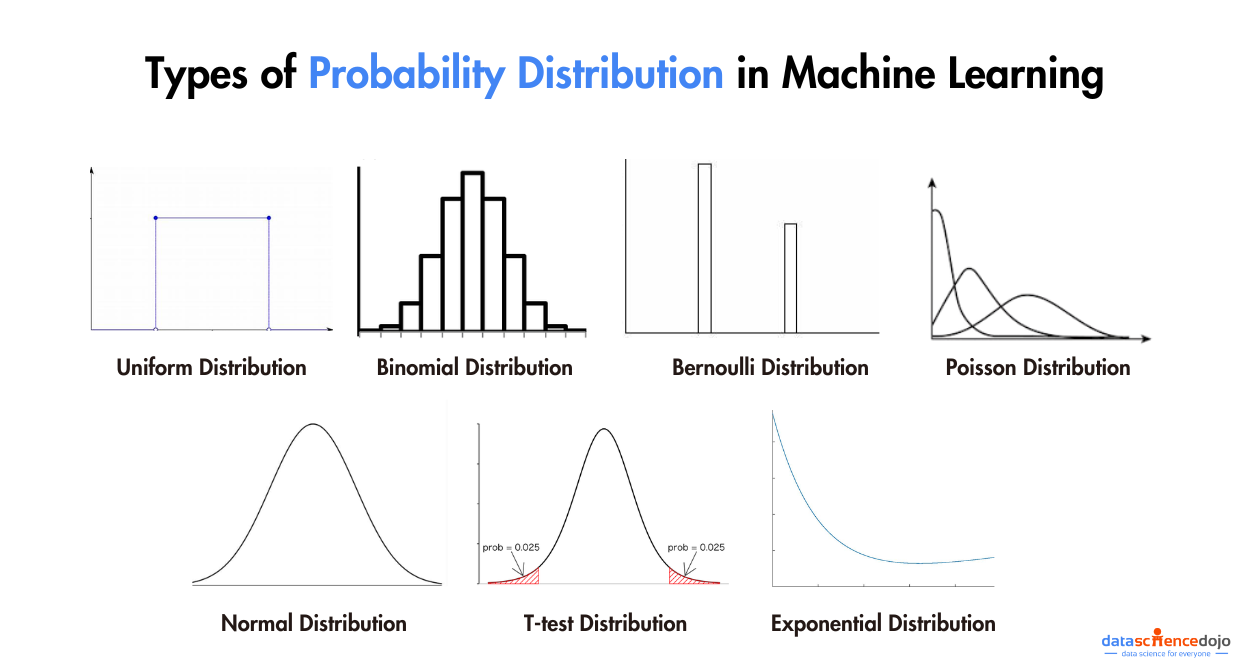
In the realm of statistics and machine learning, understanding various probability distributions is paramount. One such fundamental distribution is the Binomial Distribution.

This distribution is not only a cornerstone in probability theory but also plays a crucial role in various machine learning algorithms and applications.

In this blog, we will delve into the concept of binomial distribution, its mathematical formulation, and its significance in the field of machine learning.

What is Binomial Distribution?

The binomial distribution is a discrete probability distribution that describes the number of successes in a fixed number of independent and identically distributed Bernoulli trials.

A Bernoulli trial is a random experiment where there are only two possible outcomes:

• success (with probability ( p ))
• failure (with probability ( 1 – p ))

Mathematical Formulation

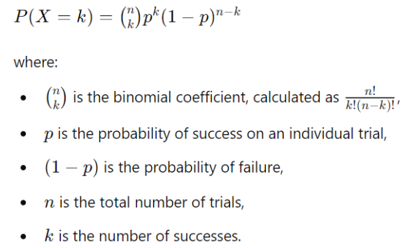
The probability of observing exactly k successes in n trials is given by the binomial probability formula:

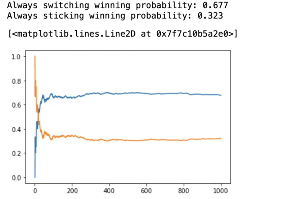
Example 1: Tossing One Coin

Let’s start with a simple example of tossing a single coin.

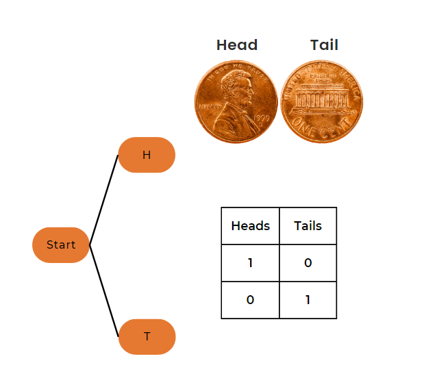
Parameters

• Number of trials (n) = 1
• Probability of heads (p) = 0.5
• Number of heads (k) = 1

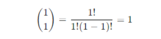
Calculation

• Binomial coefficient

• Probability

So, the probability of getting exactly one head in one toss of a coin is 0.5 or 50%.

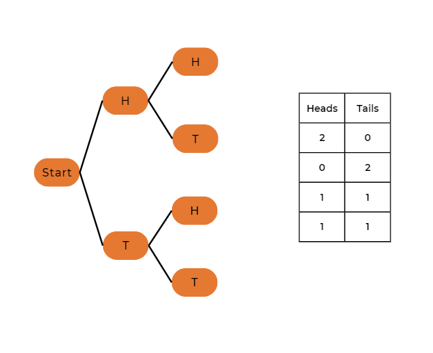
Example 2: Tossing Two Coins

Now, let’s consider the case of tossing two coins.

Parameters

• Number of trials (n) = 2
• Probability of heads (p) = 0.5
• Number of heads (k) = varies (0, 1, or 2)

Calculation for k = 0

• Binomial coefficient

• Probability

P(X = 0) = 1 × (0.5)⁰ × (1 – 0.5)² = 1 × 1 × 0.25 = 0.25

Calculation for k = 1

• Binomial coefficient

• Probability

P(X = 1) = 1 × (0.5)¹ × (1 – 0.5)¹ = 2 × 0.5 × 0.5 = 0.5

Calculation for k = 2

• Binomial coefficient

• Probability

P(X = 2) = 1 × (0.5)² × (1 – 0.5)⁰ = 1 × 0.25 × 1 = 0.25

So, the probabilities for different numbers of heads in two-coin tosses are:

• P(X = 0) = 0.25 – no heads
• P(X = 1) = 0.5 – one head
• P(X = 2) = 0.25 – two heads

Detailed Example: Predicting Machine Failure

Let’s consider a more practical example involving predictive maintenance in an industrial setting. Suppose we have a machine that is known to fail with a probability of 0.05 during a daily checkup. We want to determine the probability of the machine failing exactly 3 times in 20 days.

Step-by-Step Calculation

1. Identify Parameters

• Number of trials (n) = 20 days
• Probability of success (p) = 0.05 – failure is considered a success in this context
• Number of successes (k) = 3 failures

2. Apply the Formula

3. Compute Binomial Coefficient

4. Calculate Probability

• Plugging the values into the binomial formula

• Substitute the values

P(X = 3) = 1140 × (0.05)³ × (0.95)¹⁷

• Calculate (0.05)³

(0.05)³ = 0.000125

• Calculate (0.95)¹⁷

(0.95)¹⁷ ≈ 0.411

5. Multiply all Components Together

P(X = 3) = 1140 × 0.000125 × 0.411 ≈ 0.0585

Therefore, the probability of the machine failing exactly 3 times in 20 days is approximately 0.0585 or 5.85%. 

Role of Binomial Distribution in Machine Learning 

The binomial distribution is integral to several aspects of machine learning, providing a foundation for understanding and modeling binary events, hypothesis testing, and beyond.

Let’s explore how it intersects with various machine-learning concepts and techniques. 

Binary Classification

In binary classification problems, where the outcomes are often categorized as success or failure, the binomial distribution forms the underlying probabilistic model. For instance, if we are predicting whether an email is spam or not, each email can be thought of as a Bernoulli trial.

Algorithms like Logistic Regression and Support Vector Machines (SVM) are particularly designed to handle these binary outcomes. 

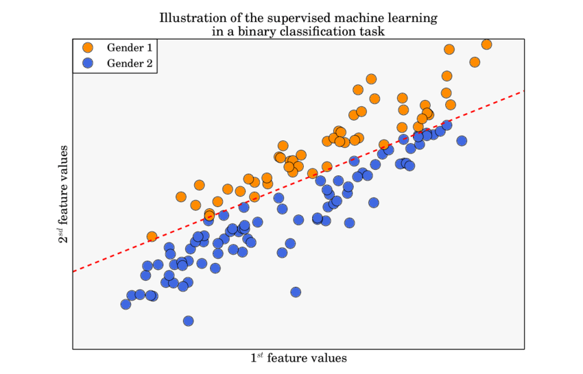
Understanding the binomial distribution helps in correctly interpreting the results of these classifiers. The performance metrics such as accuracy, precision, recall, and F1-score ultimately derive from the binomial probability model.

This understanding ensures that we can make informed decisions about model improvements and performance evaluation.

Hypothesis Testing

Statistical hypothesis testing, essential in validating machine learning models, often employs the binomial distribution to ascertain the significance of observed outcomes.

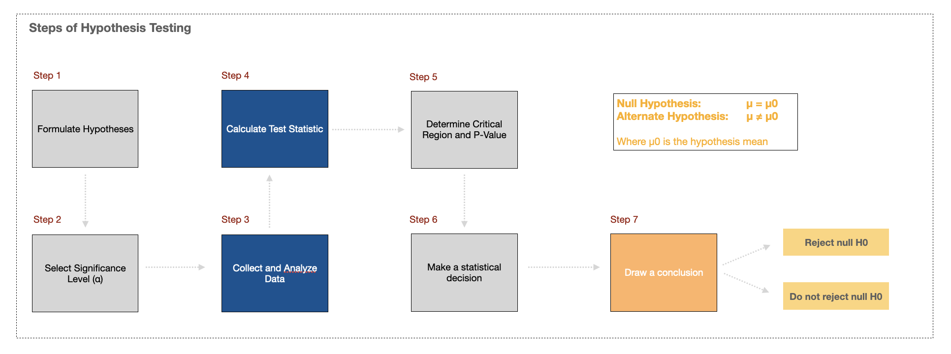
For instance, in A/B testing, which is widely used in machine learning for comparing model performance or feature impact, the binomial distribution helps in calculating p-values and confidence intervals.

You can also explore an ethical way of A/B testing

Consider an example where we want to determine if a new feature in a recommendation system improves user click-through rates. By modeling the click events as a binomial distribution, we can perform a hypothesis test to evaluate if the observed improvement is statistically significant or just due to random chance.

Generative Models

Generative models such as Naive Bayes leverage binomial distributions to model the probability of observing certain classes given specific features. This is particularly useful when dealing with binary or categorical data.

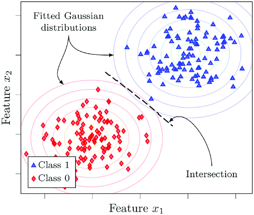
In text classification tasks, for example, the presence or absence of certain words (features) in a document can be modeled using binomial distributions to predict the document’s category (class). 

By understanding the binomial distribution, we can better grasp how these models work under the hood, leading to more effective feature engineering and model tuning. 

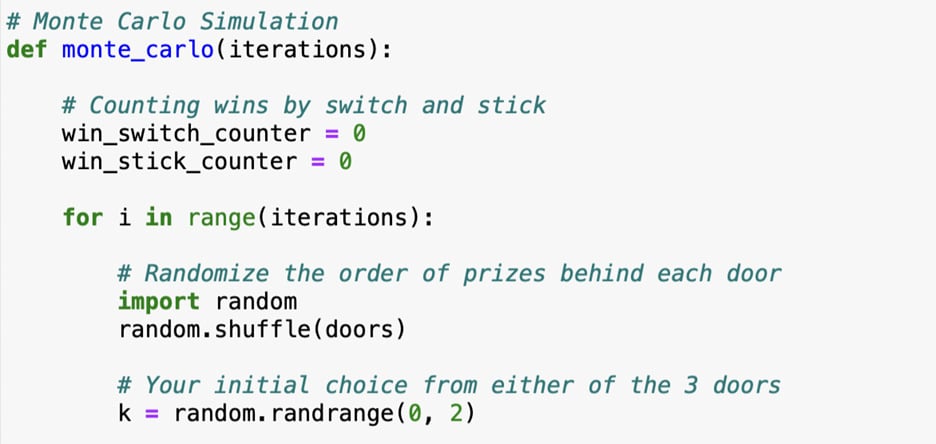
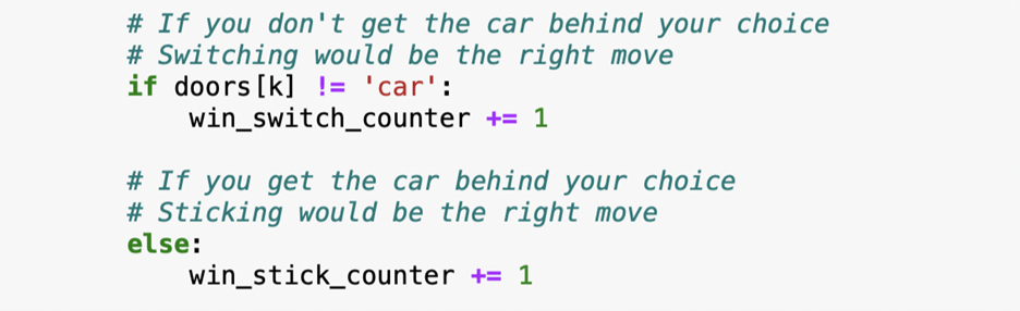
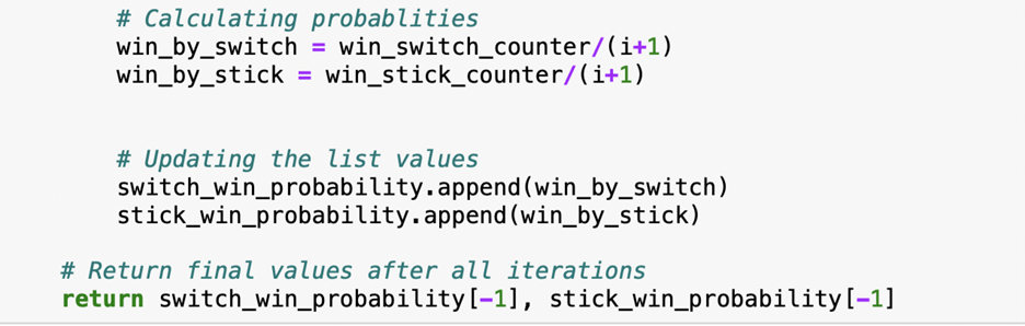
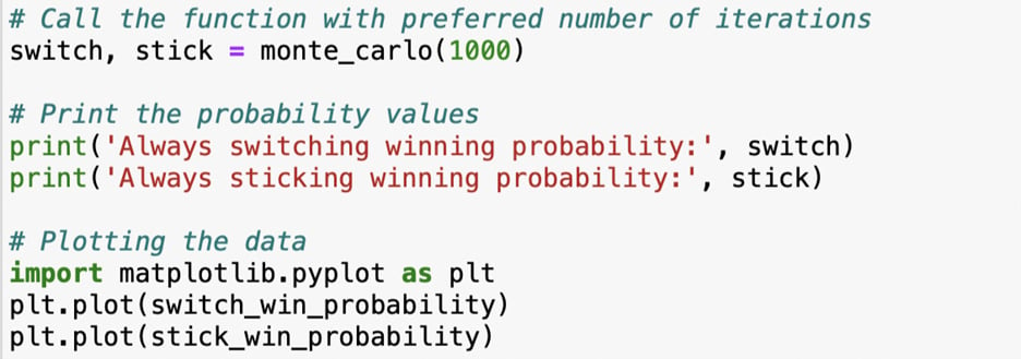
Monte Carlo Simulations

Monte Carlo simulations, which are used in various machine learning applications for uncertainty estimation and decision-making, often rely on binomial distributions to model and simulate binary events over numerous trials.

These simulations can help in understanding the variability and uncertainty in model predictions, providing a robust framework for decision-making in the presence of randomness.

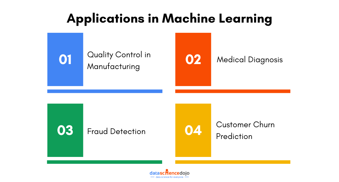
Practical Applications in Machine Learning 

Quality Control in Manufacturing

In manufacturing, maintaining high-quality standards is crucial. Machine learning models are often deployed to predict the likelihood of defects in products.

Here, the binomial distribution is used to model the number of defective items in a batch. By understanding the distribution, we can set appropriate thresholds and confidence intervals to decide when to take corrective actions.

Explore Locust – a tool for quality assurance

Medical Diagnosis

In medical diagnosis, machine learning models assist in predicting the presence or absence of a disease based on patient data. The binomial distribution provides a framework for understanding the probabilities of correct and incorrect diagnoses.

This is critical for evaluating the performance of diagnostic models and ensuring they meet the necessary accuracy and reliability standards. 

Fraud Detection

Fraud detection systems in finance and e-commerce rely heavily on binary classification models to distinguish between legitimate and fraudulent transactions. The binomial distribution aids in modeling the occurrence of fraud and helps in setting detection thresholds that balance false positives and false negatives effectively.

Learn how cybersecurity has revolutionized with the use of data science

Customer Churn Prediction

Predicting customer churn is vital for businesses to retain their customer base. Machine learning models predict whether a customer will leave (churn) or stay (retain). The binomial distribution helps in understanding the probabilities of churn events and in setting up retention strategies based on these probabilities. 

Why Use Binomial Distribution?

Binomial distribution is a fundamental concept that finds extensive application in machine learning. From binary classification to hypothesis testing and generative models, understanding and leveraging this distribution can significantly enhance the performance and interpretability of machine learning models.

By mastering the binomial distribution, you equip yourself with a powerful tool for tackling a wide range of problems in statistics and machine learning. 

Feel free to dive deeper into this topic, experiment with different values, and explore the fascinating world of probability distributions in machine learning! 

“Statistics is the grammar of science”, Karl Pearson

In the world of data science, there is a secret language that benefits those who understand it. Do you want to know what makes a data expert efficient? It’s having a profound understanding of the data. Unfortunately, you can’t have a friendly conversation with the data, but don’t worry, we have the next best solution.

Here are the top ten statistical concepts that you must have in your arsenal.  Whether you’re a budding data scientist, a seasoned professional, or merely intrigued by the inner workings of data-driven decision-making, prepare for an enthralling exploration of the statistical principles that underpin the world of data science. 

 10 statistical concepts you should know

1. Descriptive statistics: 

Starting with the most fundamental and essential statistical concept, descriptive statistics. Descriptive statistics are the specific methods and measures that describe the data. It’s like the foundation of your building. It is a sturdy groundwork upon which further analysis can be constructed. Descriptive statistics can be broken down into measures of central tendency and measures of variability. 

• Measure of Central Tendency: 

Central Tendency is defined as “the number used to represent the center or middle of a set of data values”. It is a single value that is typically representative of the whole data. They help us understand where the “average” or “central” point lies amidst a collection of data points.

There are a few techniques to find the central tendency of the data, namely “Mean” (average), “Median” (middle value when data is sorted), and “Mode” (most frequently occurring values).  

• Measures of variability: 

Measures of variability describe the spread, dispersion, and deviation of the data. In essence, they tell us how much each value point deviates from the central tendency. A few measures of variability are “Range”, “Variance”, “Standard Deviation”, and “Quartile Range”. These provide valuable insights into the degree of variability or uniformity in the data.   

 2. Inferential statistics: 

Inferential statistics enable us to draw conclusions about the population from a sample of the population. Imagine having to decide whether a medicinal drug is good or bad for the general public. It is practically impossible to test it on every single member of the population.

This is where inferential statistics comes in handy. Inferential statistics employ techniques such as hypothesis testing and regression analysis (also discussed later) to determine the likelihood of observed patterns occurring by chance and to estimate population parameters.

This invaluable tool empowers data scientists and researchers to go beyond descriptive analysis and uncover deeper insights, allowing them to make data-driven decisions and formulate hypotheses about the broader context from which the data was sampled. 

3. Probability distributions: 

Probability distributions serve as foundational concepts in statistics and mathematics, providing a structured framework for characterizing the probabilities of various outcomes in random events. These distributions, including well-known ones like the normal, binomial, and

Poisson distributions offer structured representations for understanding how data is distributed across different values or occurrences.

Much like navigational charts guiding explorers through uncharted territory, probability distributions function as reliable guides through the landscape of uncertainty, enabling us to quantitatively assess the likelihood of specific events.

They constitute essential tools for statistical analysis, hypothesis testing, and predictive modeling, furnishing a systematic approach to evaluate, analyze, and make informed decisions in scenarios involving randomness and unpredictability. Comprehension of probability distributions is imperative for effectively modeling and interpreting real-world data and facilitating accurate predictions. 

Read More —-> 7 types of statistical distributions with practical examples 

4. Sampling methods: 

We now know inferential statistics help us make conclusions about the population from a sample of the population. How do we ensure that the sample is representative of the population? This is where sampling methods come to aid us.

Sampling methods are a set of methods that help us pick our sample set out of the population. Sampling methods are indispensable in surveys, experiments, and observational studies, ensuring that our conclusions are both efficient and statistically valid. There are many types of sampling methods. Some of the most common ones are defined below. 

• Simple Random Sampling: A method where each member of the population has an equal chance of being selected for the sample, typically through random processes. 
• Stratified Sampling: The population is divided into subgroups (strata), and a random sample is taken from each stratum in proportion to its size. 
• Systematic Sampling: Selecting every “kth” element from a population list, using a systematic approach to create the sample. 
• Cluster Sampling: The population is divided into clusters, and a random sample of clusters is selected, with all members in selected clusters included. 
• Convenience Sampling: Selection of individuals/items based on convenience or availability, often leading to non-representative samples. 
• Purposive (Judgmental) Sampling: Researchers deliberately select specific individuals/items based on their expertise or judgment, potentially introducing bias. 
• Quota Sampling: The population is divided into subgroups, and individuals are purposively selected from each subgroup to meet predetermined quotas. 
• Snowball Sampling: Used in hard-to-reach populations, where participants refer researchers to others, leading to an expanding sample. 

5. Regression analysis: 

Regression analysis is a statistical method that helps us quantify the relationship between a dependent variable and one or more independent variables. It’s like drawing a line through data points to understand and predict how changes in one variable relate to changes in another.

Regression models, such as linear regression or logistic regression, are used to uncover patterns and causal relationships in diverse fields like economics, healthcare, and social sciences. This technique empowers researchers to make predictions, analyze cause-and-effect connections, and gain insights into complex phenomena. 

6. Hypothesis testing: 

Hypothesis testing is a key statistical method used to assess claims or hypotheses about a population using sample data. It’s like a process of weighing evidence to determine if there’s enough proof to support a hypothesis.

Researchers formulate a null hypothesis and an alternative hypothesis, then use statistical tests to evaluate whether the data supports rejecting the null hypothesis in favor of the alternative.

This method is crucial for making informed decisions, drawing meaningful conclusions, and assessing the significance of observed effects in various fields of research and decision-making. 

7. Data visualizations: 

Data visualization is the art and science of representing complex data in a visual and comprehensible form. It’s like translating the language of numbers and statistics into a graphical story that anyone can understand at a glance.

Effective data visualization not only makes data more accessible but also allows us to spot trends, patterns, and outliers, making it an essential tool for data analysis and decision-making. Whether through charts, graphs, maps, or interactive dashboards, data visualization empowers us to convey insights, share information, and gain a deeper understanding of complex datasets. 

Check out some of the most important plots for Data Science here. 

8. ANOVA (Analysis of variance): 

Analysis of Variance (ANOVA) is a statistical technique used to compare the means of two or more groups to determine if there are significant differences among them. It’s like the referee in a sports tournament, checking if there’s enough evidence to conclude that the teams’ performances are different.

ANOVA calculates a test statistic and a p-value, which indicates whether the observed differences in means are statistically significant or likely occurred by chance.

This method is widely used in research and experimental studies, allowing researchers to assess the impact of different factors or treatments on a dependent variable and draw meaningful conclusions about group differences. ANOVA is a powerful tool for hypothesis testing and plays a vital role in various fields, from medicine and psychology to economics and engineering. 

9. Time Series analysis: 

Time series analysis is a specialized field of statistics and data science that focuses on studying data points collected, recorded, or measured over time. It’s like examining the historical trajectory of a variable to understand its patterns and trends.

Time series analysis involves techniques for data visualization, smoothing, forecasting, and modeling to uncover insights and make predictions about future values.

This discipline finds applications in various domains, from finance and economics to climate science and stock market predictions, helping analysts and researchers understand and harness the temporal patterns within their data. 

10. Bayesian statistics: 

Bayesian statistics is a branch of statistics that takes a unique approach to probability and inference. Unlike classical statistics, which use fixed parameters, Bayesian statistics treat probability as a measure of uncertainty, updating beliefs based on prior information and new evidence.

It’s like continually refining your knowledge as you gather more data. Bayesian methods are particularly useful when dealing with complex, uncertain, or small-sample data, and they have applications in fields like machine learning, Bayesian networks, and decision analysis 

4. Chaos theory

Chaos theory is a branch of mathematics that studies the behavior of dynamic systems. It is used to model many different types of systems, such as the weather, the stock market, and the human heart.

One of the most important concepts in chaos theory is the butterfly effect. The butterfly effect states that small changes in the initial conditions of a system can lead to large changes in the long-term behavior of the system.

Example:

Suppose you have a butterfly flapping its wings in Brazil. This could cause a small change in the atmosphere, which could eventually lead to a hurricane in Florida.

Chaos theory is used in many different areas of physics, engineering, and economics. It is also used in everyday life, such as when predicting the weather and managing financial risks.

Learn about the Top 7 Statistical Techniques

Physics:

Read the Top 10 Statistics Books for Data Science

9. Information theory

Formula: H(X) = -∑p(x) log2(p(x))

Information theory is a branch of mathematics that studies the transmission and processing of information. It was developed by Claude Shannon in the mid-20th century.

One of the most important concepts in information theory is entropy. Entropy is a measure of the uncertainty in a message. The higher the entropy of a message, the more uncertain it is.

Example:

Suppose you have a coin. The entropy of the coin is 1 bit, because there are two equally likely outcomes: heads or tails.

If you flip the coin and it lands on heads, the entropy of the coin is 0, because there is only one possible outcome: heads.

Information theory is used in many different areas of communication, computer science, and statistics. It is also used in everyday life, such as when designing data compression algorithms and communication protocols.

Physics and Engineering:

Physics and Cosmology:

Finance and Economics:

17. Black-Scholes equation

Formula: ∂C/∂t + ½σ^2S^2∂^2C/∂S^2 – rC = 0

The Black-Scholes equation is a differential equation that describes the price of a European option. A European option is a financial contract that gives the holder the right, but not the obligation, to buy or sell an asset at a certain price on a certain date.

The Black-Scholes equation is used to price options and to develop hedging strategies. It is one of the most important equations in finance.

Example:

Suppose you are buying a call option on a stock. The Black-Scholes equation can be used to calculate the price of the call option. This information can then be used to decide whether or not to buy the call option and to determine how much to pay for it.

The Black-Scholes equation is used by many different financial institutions, such as investment banks and hedge funds. It is also used by individual investors to make investment decisions.

Probability is a fundamental concept in data science. It provides a framework for understanding and analyzing uncertainty, which is an essential aspect of many real-world problems. In this blog, we will discuss the importance of probability in data science, its applications, and how it can be used to make data-driven decisions. 

What is probability? 

It is a measure of the likelihood of an event occurring. It is expressed as a number between 0 and 1, with 0 indicating that the event is impossible and 1 indicating that the event is certain. For example, the probability of rolling a six on a fair die is 1/6 or approximately 0.17. 

In data science, it is used to quantify the uncertainty associated with data. It helps data scientists to make informed decisions by providing a way to model and analyze the variability of data. It is also used to build models that can predict future events or outcomes based on past data. 

Applications of probability in data science 

There are many applications of probability in data science, some of which are discussed below: 

1. Statistical inference:

Statistical inference is the process of drawing conclusions about a population based on a sample of data. It plays a central role in statistical inference by providing a way to quantify the uncertainty associated with estimates and hypotheses. 

2. Machine learning:

Machine learning algorithms make predictions about future events or outcomes based on past data. For example, a classification algorithm might use probability to determine the likelihood that a new observation belongs to a particular class. 

3. Bayesian analysis:

Bayesian analysis is a statistical approach that uses probability to update beliefs about a hypothesis as new data becomes available. It is commonly used in fields such as finance, engineering, and medicine. 

4. Risk assessment:

It is used to assess risk in many industries, including finance, insurance, and healthcare. Risk assessment involves estimating the likelihood of a particular event occurring and the potential impact of that event. 

5. Quality control:

It is used in quality control to determine whether a product or process meets certain specifications. For example, a manufacturer might use probability to determine whether a batch of products meets a certain level of quality.

6. Anomaly detection

Probability is used in anomaly detection to identify unusual or suspicious patterns in data. By modeling the normal behavior of a system or process using probability distributions, any deviations from the expected behavior can be detected as anomalies. This is valuable in various domains, including cybersecurity, fraud detection, and predictive maintenance.

How probability helps in making data-driven decisions 

It help data scientists to make data-driven decisions by providing a way to quantify the uncertainty associated with data. By using  to model and analyze data, data scientists can: 

• Estimate the likelihood of future events or outcomes based on past data. 
• Assess the risk associated with a particular decision or action. 
• Identify patterns and relationships in data. 
• Make predictions about future trends or behavior. 
• Evaluate the effectiveness of different strategies or interventions. 

Bayes’ theorem and its relevance in data science 

Bayes’ theorem, also known as Bayes’ rule or Bayes’ law, is a fundamental concept in probability theory that has significant relevance in data science. It is named after Reverend Thomas Bayes, an 18th-century British statistician and theologian, who first formulated the theorem. 

At its core, Bayes’ theorem provides a way to calculate the probability of an event based on prior knowledge or information about related events. It is commonly used in statistical inference and decision-making, especially in cases where new data or evidence becomes available. 

The theorem is expressed mathematically as follows: 

P(A|B) = P(B|A) * P(A) / P(B) 

Where: 

• P(A|B) is the probability of event A occurring given that event B has occurred. 
• P(B|A) is the probability of event B occurring given that event A has occurred. 
• P(A) is the prior probability of event A occurring. 
• P(B) is the prior probability of event B occurring. 

In data science, Bayes’ theorem is used to update the probability of a hypothesis or belief in light of new evidence or data. This is done by multiplying the prior probability of the hypothesis by the likelihood of the new evidence given that hypothesis.

Master Naive Bayes for powerful data analysis. Read this blog to understand valuable insights from your data!

For example, let’s say we have a medical test that can detect a certain disease, and we know that the test has a 95% accuracy rate (i.e., it correctly identifies 95% of people with the disease and 5% of people without it). We also know that the prevalence of the disease in the population is 1%. If we administer the test to a person and they test positive, we can use Bayes’ theorem to calculate the probability that they actually have the disease. 

In conclusion, Bayes’ theorem is a powerful tool for probabilistic inference and decision-making in data science. Incorporating prior knowledge and updating it with new evidence, it enables more accurate and informed predictions and decisions. 

Common mistakes to avoid in probability analysis 

Probability analysis is an essential aspect of data science, providing a framework for making informed predictions and decisions based on uncertain events. However, even the most experienced data scientists can make mistakes when applying probability analysis to real-world problems. In this article, we’ll explore some common mistakes to avoid: 

• Assuming independence: One of the most common mistakes is assuming that events are independent when they are not. For example, in a medical study, we may assume that the likelihood of developing a certain condition is independent of age or gender, when in reality these factors may be highly correlated. Failing to account for such dependencies can lead to inaccurate results. 
• Misinterpreting probability: Some people may think that a probability of 0.5 means that an event is certain to occur, when in fact it only means that the event has an equal chance of occurring or not occurring. Properly understanding and interpreting probability is essential for accurate analysis. 
• Neglecting sample size: Sample size plays a critical role in probability analysis. Using a small sample size can lead to inaccurate results and incorrect conclusions. On the other hand, using an excessively large sample size can be wasteful and inefficient. Data scientists need to strike a balance and choose an appropriate sample size based on the problem at hand. 
• Confusing correlation and causation: Another common mistake is confusing correlation with causation. Just because two events are correlated does not mean that one causes the other. Careful analysis is required to establish causality, which can be challenging in complex systems. 
• Ignoring prior knowledge: Bayesian probability analysis relies heavily on prior knowledge and beliefs. Failing to consider prior knowledge or neglecting to update it based on new evidence can lead to inaccurate results. Properly incorporating prior knowledge is essential for effective Bayesian analysis. 
• Overreliance on models: The models can be powerful tools for analysis, but they are not infallible. Data scientists need to exercise caution and be aware of the assumptions and limitations of the models they use. Blindly relying on models can lead to inaccurate or misleading results. 

Conclusion 

Probability is a powerful tool for data scientists. It provides a way to quantify uncertainty and make data-driven decisions. By understanding the basics of probability and its applications in data science, data scientists can build models and make predictions that are both accurate and reliable. As data becomes increasingly important in all aspects of our lives, the ability to use it effectively will become an essential skill for success in many fields. 

The Monte Carlo method is a technique for solving complex problems using probability and random numbers. Through repeated random sampling, Monte Carlo calculates the probabilities of multiple possible outcomes occurring in an uncertain process.  

Whenever you try to solve problems in the future, you make certain assumptions. For example, forecasting problems make certain assumptions like the cost of a particular item, the value of stocks, or electricity units used in the future. Since these problems try to predict an estimate of an unknown value based on historical data, there always exists inherent risk and uncertainty.  

The Monte Carlo simulation allows us to see all the possible outcomes of our decisions and assess risk, consequently allowing for better decision-making under uncertainty. 

This blog will walk through the famous Monty Hall problem, and how it can be solved using the Monte Carlo method using Python.  

Monty Hall problem 

In the Monty Hall problem, the TV show host Monty presents three doors to the participant. Behind one of the doors is a valuable prize like a car, while behind the others is a less valuable prize like a goat.  

Consider yourself to be one of the participants in the show. You choose one out of the three doors. Before opening your chosen door, Monty opens another door behind which would be one of the goats. Now you are left with two doors, behind one could be the car, and behind the other would be the other goat. 

Monty then gives you the option to either switch your answer to the other unopened door or stick to the original one.  

Is it in your favor to switch your answer to the other door? Well, probability says it is!  

Let’s see how: 

Initially, there are three unopen doors in front of you. The probability of the car being behind any of these doors is 1/3.  

Let’s say you decide to pick door #1 as the probability is the same (1/3) for each of these doors. In other words, the probability that the car is behind door #1 is 1/3, and the probability that it will be behind either door #2 or door #3 is 2/3. 

Monty is aware of the prize behind each door. He chooses to open door #3 and reveal a goat. He then asks you if you would like to either switch to door #2 or stick with door #1.  

To solve the problem, let’s switch to Python and apply the Monte Carlo simulation. 

Solving with Python 

Initialize the 3 prizes

Create python lists to store the probabilities after each game. We will play as many games as iterations input.  

Monte Carlo simulation 

Before starting the game, we randomize the prizes behind each door. One of the doors will have a car behind it, while the other two will have a goat each. When we play a large number of games, all possible permutations get covered of prize distributions, and door choices get covered.  

Below is the code that decides if your choice was correct or not, and if switching would’ve been the correct move.  

 After playing each game, the winning probabilities are updated and stored in the lists. When all games have been played, we return the final values of each of the lists, i.e., winning by switching your choice and winning by sticking to your choice.  

Get results

Enter your desired number of iterations (the higher the number, the more numbers of games will be played to approximate the probabilities). In the final step, plot your results.  

After running the simulation 1000 times, the probability that we win by always switching is 67.7%, and the probability that we win by always sticking to our choice is 32.3%. In other words, you will win approximately 2/3 times if you switch your door, and only 1/3 times if you stick to the original door. 

Therefore, according to the Monte Carlo simulation, we are confident that it works to our advantage to switch the door in this tricky game. 

Written by Aadam Nadeem