If you’re enthusiastic to learn Naive Bayes and want to go more in-depth with a step-by-step example, look no further and read along.
A deep dive into Naïve Bayes for text classification
Naive Bayes is one of the most common machine learning algorithms that is often used for classifying text into categories. Naive Bayes is a probabilistic classification algorithm as it uses probability to make predictions for the purpose of classification. If you are new to machine learning, Naive Bayes is one of the easiest classification algorithms to get started with.
In part 1 of this two-part series, we will dive deep into the theory of Naïve Bayes and the steps in building a model, using an example of classifying text into positive and negative sentiment. In part 2, we will dive even deeper into Naïve Bayes, digging into the underlying probability. For those of you who are enthusiastic to learn this common algorithm and want to go more in-depth with a step-by-step example, this is the blog for you!
Training phase of the Naïve Bayes model
Let’s say there is a restaurant review, “Very good food and service!!!”, and you want to predict that whether this given review implies a positive or a negative sentiment. To do this, we will first need to train a model (which essentially means to determine counts of words of each category) on a relevant labelled training dataset. New reviews are then classified into one of the given sentiments (positive or negative) using the trained model.
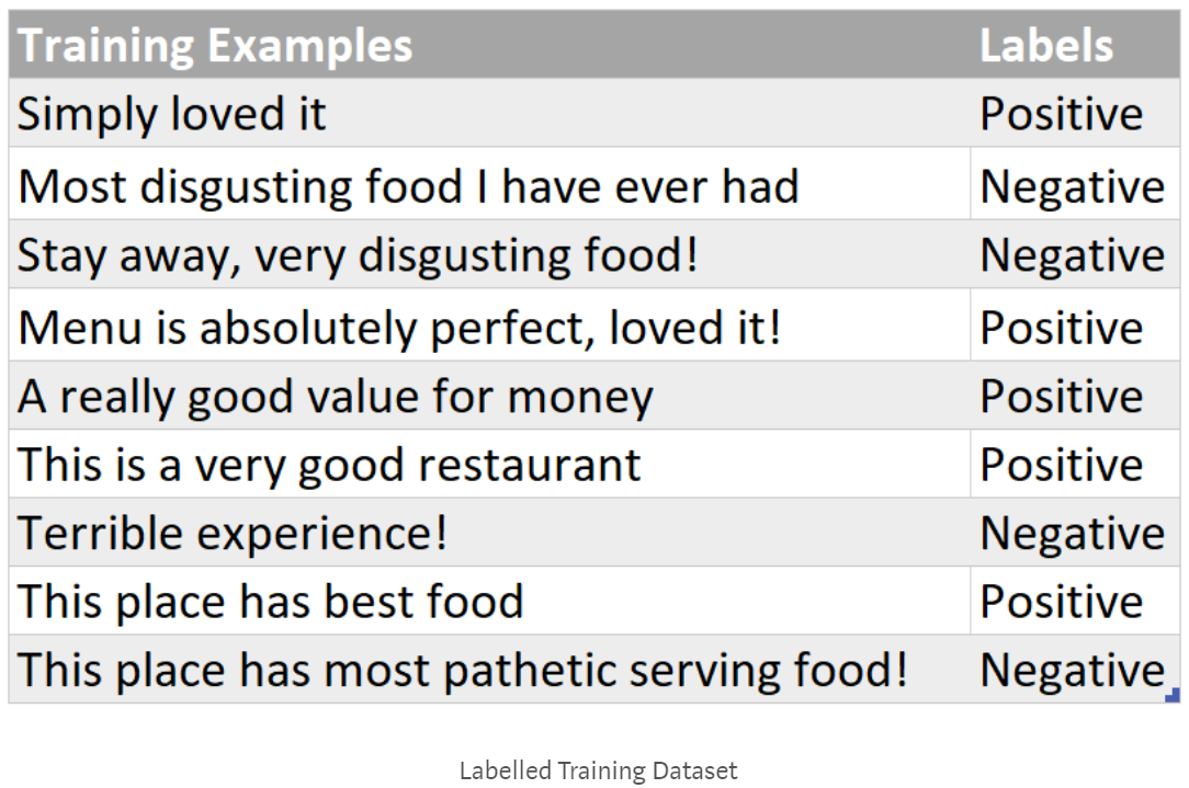
Let’s say you are given a training dataset that looks something like the below (a review and its corresponding sentiment):
A quick side note: Naive Bayes classifier is a supervised machine learning algorithm in that it learns the features that map back to a labeled outcome.
Let’s begin!
Step 1: Data pre-processing
As part of the pre-processing phase, all words in the corpus/dataset are converted to lowercase and everything apart from letters and numbers (e.g. punctuation and special characters) is removed from the text.For example:
Tokenize each sentence or piece of text by splitting it into words, using whitespace to split/separate the text into each word. For example:
Keep each tokenized sentence or piece of text in its own item within a list, so that each item in the list is a sentence broken up into words.
Each word in the vocabulary of each class of the train set constitutes a categorical feature. This implies that counts of all the unique words (i.e. vocabulary/vocab) of each class are basically a set of features for that particular class. Counts are useful because we need a numeric representation of the categorical word features as the Naive Bayes Model/Algorithm requires numeric features to find out the probabilistic scores.
Lastly, split the list of tokenized sentences or pieces of text into a train and test subset. A good rule of thumb is to split by 70/30 – 70% of sentences randomly selected for the train set, and the remaining 30% for the test set.
Step 2: Training your Naïve Bayes model
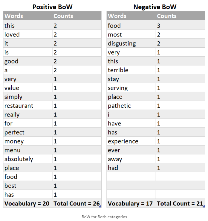
Now we simply make two bag of words (BoW), one for each category. Each of bag of words simply contains words and their corresponding counts. All words belonging to the ‘Positive’ sentiment/label will go to one BoW and all words belonging to the ‘Negative’ sentiment will have their own BoW. Every sentence in training set is split into words and this is how simply word-count pairs are constructed as demonstrated below:
Great! You have achieved two major milestones – text pre-processing/cleaning and training the Naïve Bayes model!
Now let’s move onto the most essential part of building the Naive Bayes model for text classification – i.e. using the above trained model to predict new restaurant reviews.
Testing phase – Where prediction comes into play!
Let’s say your model is given a new restaurant review, “Very good food and service!!!”, and it needs to classify to which category it belongs to. Does it belong to positive review or a negative one? We need to find the probability of this given review of belonging to each category and then assign it either a positive or a negative label depending upon which particular category this test example was able to score more probability.
Finding the probability of a given test example
*A quick side note: Your test set should have gone through the same text pre-processing as applied to the train set. *
Step 1: Understanding how probability predicts the label for test example
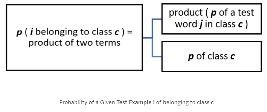
Here is the not-so-intimidating mathematical form of finding the probability of a piece of text belonging to a class:
• i is the test example, so “Very good food and service!!!”• The total number of words in i is 5, so values of j (representing the feature number) vary from 1 to 5
Let’s map the above scenario to the given test example to make it more clear!
Step 2: Finding Value of the Term — p of class c
Step 3: Finding value of term: product (p of a test word j in class c)
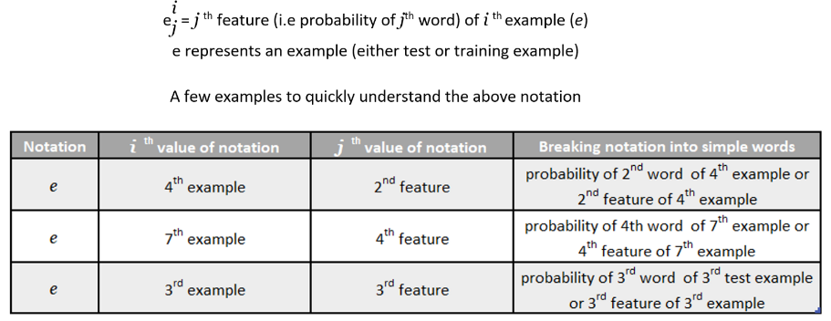
Before we start deducing probability of a test word j in a specific class c let’s quickly get familiar with some easy-peasy notation that is being used in the not so distant lines of this blog post:
i = 1, as we have only one example in our test set at the moment (for the sake of understanding).
A quick side note: During test time/prediction time, we map every word from the test example to its count that was found during the training phase. In this case, we are looking for 5 total word counts for this given test example.
Still with me? Let’s take a short break. Here’s a random, cute cat:
Finding the probability of a test word “j” in class c
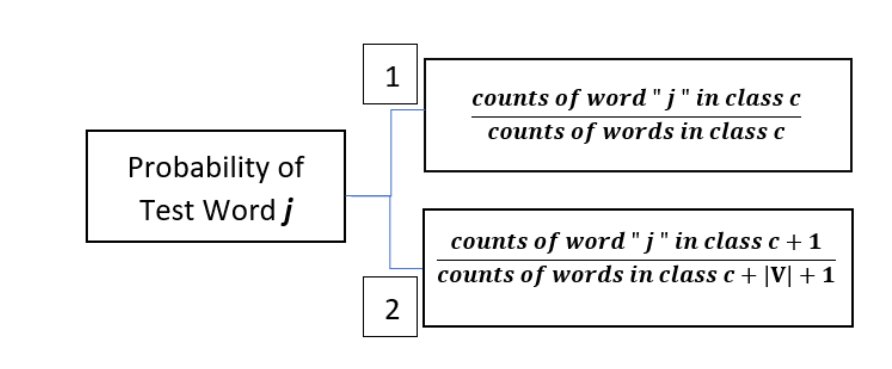
Before we start calculating the product (p of a test word “j” in class c), we obviously first need to determine p of a test word “j” in class c. There are two ways of doing this as specified below:
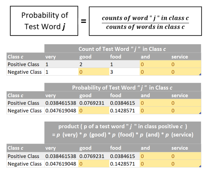
Let’s try finding probabilities using method 1, as it is more practically used in the field.
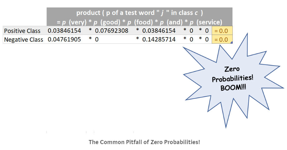
Now we can multiply the probabilities of individual words (as found above) in order to find the numerical value of the term: product (p of a test word “j” in class c)
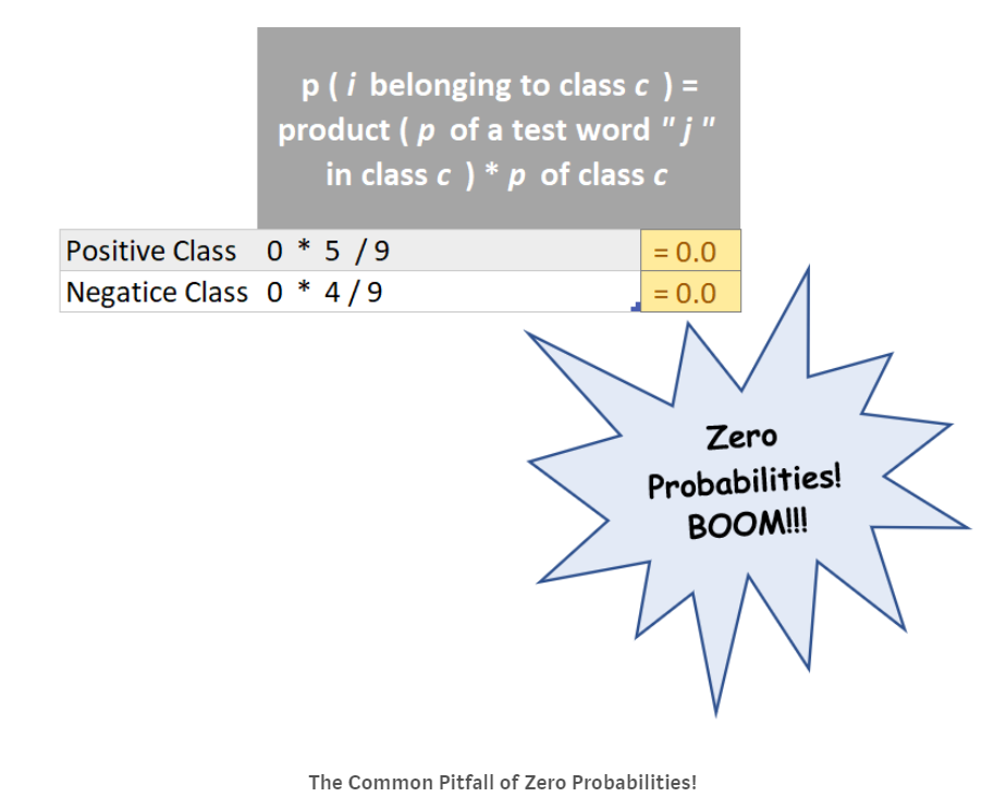
Now we have numerical values for both the terms i.e. (p of class c and product (p of a test word “j” in class c)) in both the classes. So we can multiply both of these terms in order to determine p (i belonging to class c) for both the categories. This is demonstrated below:
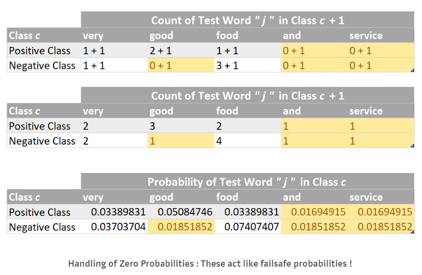
The p (i belonging to class c) is zero for both the categories, but clearly the test example “Very good food and service!!!” belongs to positive class. So there’s a problem here. This problem happened because the product (p of a test word “j” in class c) was zero for both the categories and this in turn was zero because a few words in the given test example (highlighted in orange) NEVER EVER appeared in our training dataset and hence their probability was zero! Clearly, they have caused all the destruction!
So does this imply that whenever a word that appears in the test example but never ever occurred in the training dataset it will always cause such destruction? And in such case our trained model will never be able to predict the correct sentiment? Will it just randomly pick a positive or negative category since both have the same zero probability and predict wrongly? The answer is NO! This is where the second method (numbered 2) comes into play. Method 2 is actually used to deduce p(i belonging to class c). But before we move on to method number 2, we should first get familiar with its mathematical brainy stuff!
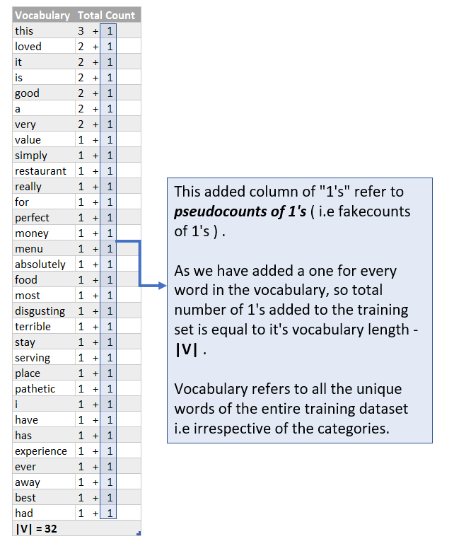
After adding pseudo-counts of 1s, the probability p of a test word that never appeared in the training dataset will not default to zero and therefore, the numerical value of the term product (p of a test word “j” in class c) will also not end up as a zero, which in turn p (i belonging to class c) will not be zero. So all is well and there is no more destruction by zero probabilities!
The numerator term of method number 2 will have an added, 1 as we have added a 1 for every word in the vocabulary and so it becomes:
Total count of word “j” in class c = count of word “j” in class c + 1
Similarly, the denominator becomes:Total counts of words in class c = count of words in class c + |V| + 1
And so the complete formula becomes:
Total count of word “j” in class c = 0 + 1
So any unknown word in the test set will have the following probability:
Why add 1 to the denominator?
We are considering that there are no more unknown test words. The numerator will always be “1” even when a word that never occurred in the training dataset occurs in the test set. In other words, we are assuming that an unknown test word occurred once (i.e. it’s count is 1) and so this also needs to be adjusted in the denominator. This is like adding the unknown word to the vocabulary of your training dataset, implying that the total count will be |V| + 1.
Now take the time to give yourself a pat on the back for getting this far! You still have little bit to go in finding the probabilities and completing the testing phase. You are almost there.
Finding the probabilities using method 2
Now as the probability of the test example “Very good food and service!!!” is more for the positive class (i.e. 9.33E-09) as compared to the negative class (i.e. 7.74E-09), so we can predict it as a Positive Sentiment! And that is how we simply predict a label for a test/unseen example.
A quick side note: As like every other machine learning algorithm, Naive Bayes too needs a validation set to assess the trained model’s effectiveness. But we deliberately jumped to the testing part in order to demonstrate a basic implementation of Naive Bayes.
Continue learning with Part 2.
This blog was originally published on towardsdatascience.com
Written by Aisha Jawed


