Unlock your data science potential and transform your career.
Join our Data Science Bootcamp today and get 25% off!

encoding

Data is a crucial element of modern-day businesses. With the growing use of machine learning (ML) models to handle, store, and manage data, the efficiency and impact of enterprises have also increased. It has led to advanced techniques for data management, where each tactic is based on the type of data and the way to handle it.

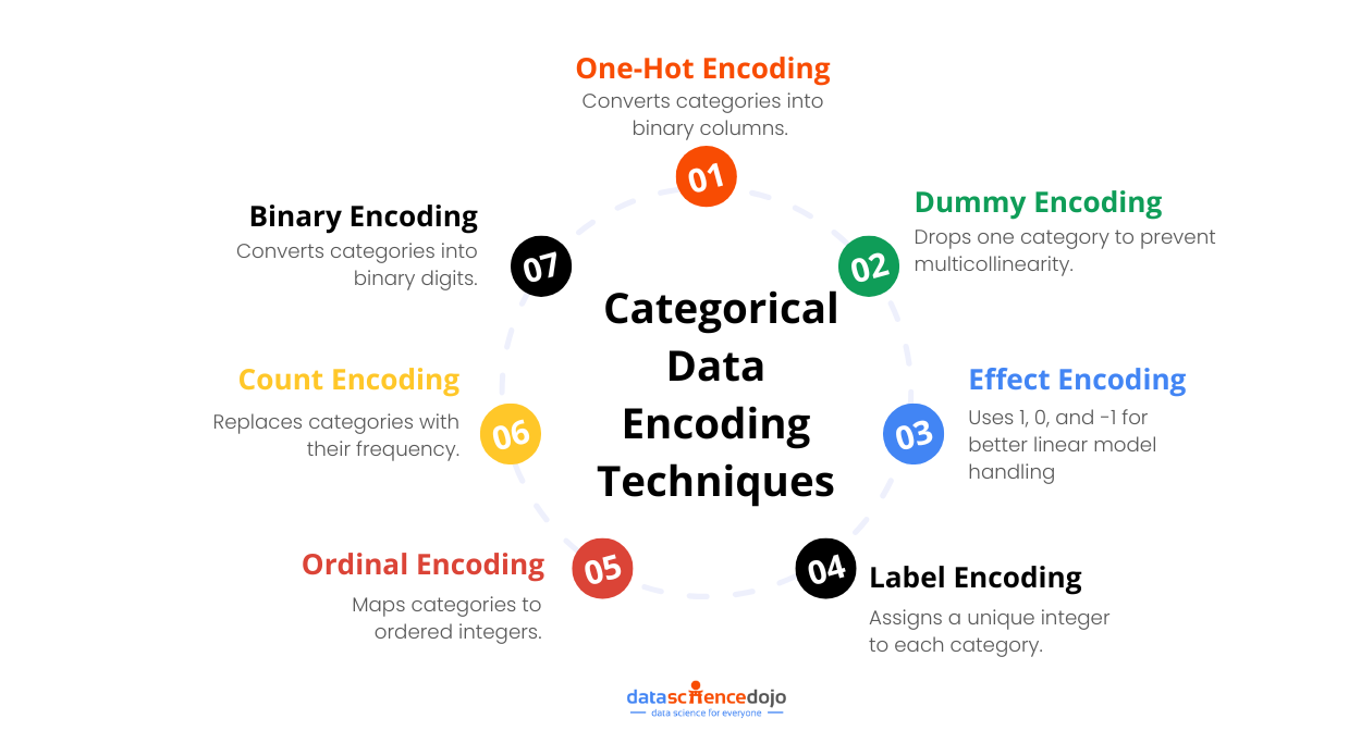
Categorical data is one such form of information that is handled by ML models using different methods. In this blog, we will explore the basics of categorical data. We will also explore the 7 main encoding methods used to process categorical data.


LLM bootcamp banner


What is Categorical Data?

Categorical data, also known as nominal or ordinal data, consists of values that fall into distinct categories or groups. Unlike numerical data, which represents measurable quantities, categorical data represents qualitative or descriptive characteristics. These variables can be represented as strings or labels and have a finite number of possible values.

Examples of Categorical Data

  • Nominal Data: Categories that do not have an inherent order or ranking. For instance, the city where a person lives (e.g., Delhi, Mumbai, Ahmedabad, Bangalore).
  • Ordinal Data: Categories that have an inherent order or ranking. For example, the highest degree a person has (e.g., High School, Diploma, Bachelor’s, Master’s, Ph.D.).
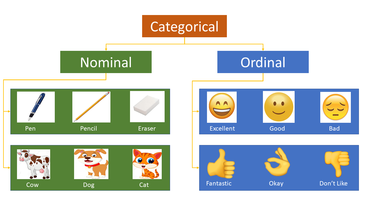
 

Categorical data encoding - types of categorical data
Types of categorical data – Source: LinkedIn


Importance of Categorical Data in Machine Learning

Categorical data is crucial in machine learning for several reasons. ML models often require numerical input, so categorical data must be converted into a numerical format for effective processing and analysis. Here are some key points highlighting the importance of categorical data in machine learning:

1. Model Compatibility

Most machine learning algorithms work with numerical data, making it essential to transform categorical variables into numerical values. This conversion allows models to process the data and extract valuable information.

2. Pattern Recognition

Encoding categorical data helps models identify patterns within the data. For instance, specific categories might be strongly associated with particular outcomes, and recognizing these patterns can improve model accuracy and predictive power.

3. Bias Prevention

Proper encoding ensures that all features are equally weighted, preventing bias. For example, one-hot encoding and other methods help avoid unintended biases that might arise from the categorical nature of the data.

4. Feature Engineering

Encoding categorical data is a crucial part of feature engineering, which involves creating features that make ML models more effective. Effective feature engineering, including proper encoding, can significantly enhance model performance.


Learn about 101 ML algorithms for data science with cheat sheets


5. Handling High Cardinality

Advanced encoding techniques like target encoding and hashing are used to manage high cardinality features efficiently. These techniques help reduce dimensionality and computational complexity, making models more scalable and efficient.

6. Avoiding the Dummy Variable Trap

While techniques like one-hot encoding are popular, they can lead to issues like the dummy variable trap, where features become highly correlated. Understanding and addressing these issues through proper encoding methods is essential for robust model performance.

7. Improving Model Interpretability

Encoded categorical data can make models more interpretable. For example, target encoding provides a direct relationship between the categorical feature and the target variable, making it easier to understand how different categories influence the model’s predictions.

Let’s take a deeper look into 7 main encoding techniques for categorical data.

1. One-Hot Encoding

One-hot encoding, also known as dummy encoding, is a popular technique for converting categorical data into a numerical format. This technique is particularly suitable for nominal categorical features where the categories have no inherent order or ranking.


Categorical data encoding - one-hot encoding
An example of one-hot encoding – Source: ResearchGate


How One-Hot Encoding Works?

  1. Determine the categorical feature in your dataset that needs to be encoded.
  2. For each unique category in the feature, create a new binary column.
  3. Assign 1 to the column that corresponds to the category of the data point and 0 to all other new columns.

Advantages of One-Hot Encoding

  1. Preserves Information: Maintains the distinctiveness of labels without implying any ordinality.
  2. Compatibility: Provides a numerical representation of categorical data, making it suitable for many machine learning algorithms.

Use Cases

  1. Nominal Data: When dealing with nominal data where categories have no meaningful order. For example, in a dataset containing the feature “Type of Animal” with categories like “Dog”, “Cat”, and “Bird”, one-hot encoding is ideal because there is no inherent ranking among the animals 2.
  2. Machine Learning Models: Particularly beneficial for algorithms that cannot handle categorical data directly, such as linear regression, logistic regression, and neural networks.
  3. Handling Missing Values: One-hot encoding handles missing values efficiently. If a category is absent, it results in all zeros in the one-hot encoded columns, which can be useful for certain ML models.

Challenges with One-Hot Encoding

  1. Curse of Dimensionality: It can lead to a high number of new columns (dimensions) in your dataset, increasing computational complexity and storage requirements.
  2. Multicollinearity: The newly created binary columns can be correlated, which can be problematic for some models that assume independence between features.
  3. Data Sparsity: One-hot encoding can result in sparse matrices where most entries are zeros, which can be memory-inefficient and affect model performance.

Hence, one-hot encoding is a powerful and widely used technique for converting categorical data into a numerical format, especially for nominal data. Understanding when and how to use one-hot encoding is crucial for effective feature engineering in machine learning projects.

2. Dummy Encoding

Dummy encoding is a technique for converting categorical variables into a numerical format by transforming them into a set of binary variables.

It is similar to one-hot encoding but with a key distinction: dummy encoding uses (N-1) binary variables to represent (N) categories, which helps to avoid multicollinearity issues commonly known as the dummy variable trap.
 

Categorical data encoding - dummy encoding
An example of dummy encoding – Source: Medium


How Dummy Encoding Works?

Dummy encoding transforms each category in a categorical feature into a binary column, but it drops one category. The process can be explained as follows:

  1. Determine the categorical feature in your dataset that needs to be encoded.
  2. For each unique category in the feature (except one), create a new binary column.
  3. Assign 1 to the column that corresponds to the category of the data point and 0 to all other new columns.

Advantages of Dummy Encoding

  1. Avoids Multicollinearity: By dropping one category, dummy encoding prevents the dummy variable trap where one column can be perfectly predicted from the others.
  2. Preserves Information: Maintains the distinctiveness of labels without implying any ordinality.

Use Cases

  1. Regression Models: Suitable for regression models where multicollinearity can be a significant issue. By using (N-1) binary variables for (N) categories, dummy encoding helps to avoid this problem.
  2. Nominal Data: When dealing with nominal data where categories have no meaningful order, dummy encoding is ideal. For example, in a dataset containing the feature “Department” with categories like “Finance”, “HR”, and “IT”, dummy encoding can be used to convert these categories into binary columns.

Challenges with Dummy Encoding

  1. Curse of Dimensionality: Similar to one-hot encoding, dummy encoding can lead to a high number of new columns (dimensions) in your dataset, increasing computational complexity and storage requirements.
  2. Data Sparsity: Dummy encoding can result in sparse matrices where most entries are zeros, which can be memory-inefficient and affect model performance.

However, dummy encoding is a useful technique for encoding categorical data. You must carefully choose this technique based on the details of your ML project.


Also read about rank-based encoding


3. Effect Encoding

Effect encoding, also known as Deviation Encoding or Sum Encoding, is an advanced categorical data encoding technique. It is similar to dummy encoding but with a key difference: instead of using binary values (0 and 1), effect encoding uses three values: 1, 0, and -1.

This encoding is particularly useful when dealing with categorical variables in linear models because it helps to handle the multicollinearity issue more effectively.
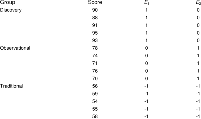
 

Categorical data encoding - effect encoding
An example of effect encoding – Source: ResearchGate


How Effect Encoding Works?

In effect encoding, the categories of a feature are represented using 1, 0, and -1. The idea is to represent the absence of the first category (baseline category) by -1 in all corresponding binary columns.

  1. Determine the categorical feature in your dataset that needs to be encoded.
  2. For each unique category in the feature (except one), create a new binary column.
  3. Assign 1 to the column that corresponds to the category of the data point, 0 to all other new columns, and -1 to the row that would otherwise be all 0s in dummy encoding.

Advantages of Effect Encoding

  1. Avoids Multicollinearity: By using -1 in place of the baseline category, effect encoding helps to handle multicollinearity better than dummy encoding.
  2. Interpretable Coefficients: In linear models, the coefficients of effect-encoded variables are interpreted as deviations from the overall mean, which can sometimes make the model easier to interpret.

Use Cases

  1. Linear Models: When using linear regression or other linear models, effect encoding helps to handle multicollinearity issues effectively and makes the coefficients more interpretable.
  2. ANOVA (Analysis of Variance): Effect encoding is often used in ANOVA models for comparing group means.

Thus, effect encoding is an advanced technique for encoding categorical data, particularly beneficial for linear models due to its ability to handle multicollinearity and make coefficients interpretable.

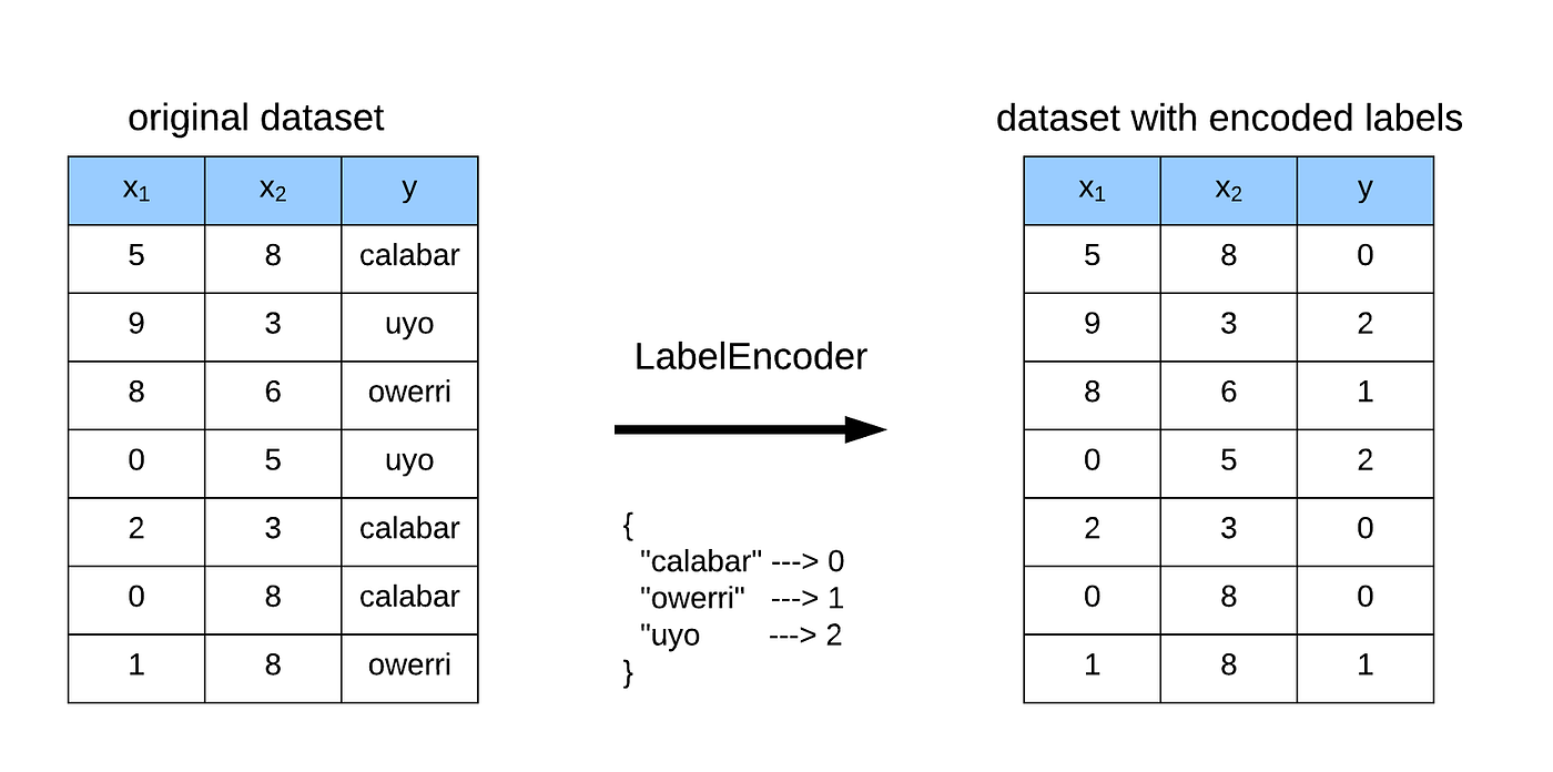
4. Label Encoding

Label encoding is a technique used to convert categorical data into numerical data by assigning a unique integer to each category within a feature. This method is particularly useful for ordinal categorical features where the categories have a meaningful order or ranking.

By converting categories to numbers, label encoding makes categorical data compatible with machine learning algorithms that require numerical input.
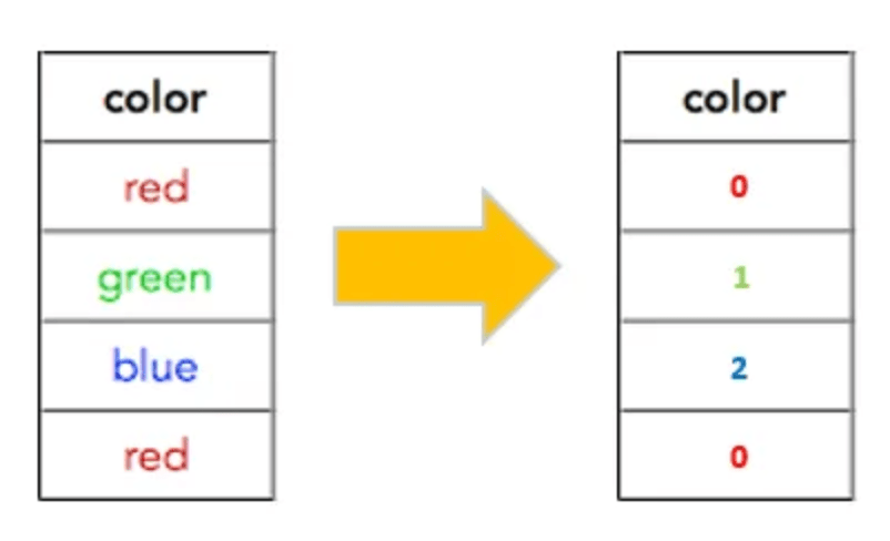
 

Categorical data encoding - label encoding
An example of label encoding – Source: Medium


How Label Encoding Works?

Label encoding assigns a unique integer to each category in a feature. The integers are typically assigned in alphabetical order or based on their appearance in the data. For ordinal features, the integers represent the order of the categories.

  1. Determine the categorical feature in your dataset that needs to be encoded.
  2. Assign a unique integer to each category in the feature.
  3. Replace the original categories in the feature with their corresponding integer values.

Advantages of Label Encoding

  1. Simple and Efficient: It is straightforward and computationally efficient.
  2. Maintains Ordinality: It preserves the order of categories, which is essential for ordinal features.

Use Cases

  1. Ordinal Data: When dealing with ordinal features where the categories have a meaningful order. For example, education levels such as “High School”, “Bachelor’s Degree”, “Master’s Degree”, and “PhD” can be encoded as 0, 1, 2, and 3, respectively.
  2. Tree-Based Algorithms: Algorithms like decision trees and random forests can handle label-encoded data well because they can naturally work with the integer representation of categories.

Challenges with Label Encoding

  1. Unintended Ordinality: When used with nominal data (categories without a meaningful order), label encoding can introduce unintended ordinality, misleading the model to assume some form of ranking among the categories.
  2. Model Bias: Some machine learning algorithms might misinterpret the integer values as having a mathematical relationship, potentially leading to biased results.

Label encoding is a simple yet powerful technique for converting categorical data into numerical format, especially useful for ordinal features. However, it should be used with caution for nominal data to avoid introducing unintended relationships.

By following these guidelines and examples, you can effectively implement label encoding in your ML workflows to handle categorical data efficiently.

5. Ordinal Encoding

Ordinal encoding is a technique used to convert categorical data into numerical data by assigning a unique integer to each category within a feature, based on a meaningful order or ranking. This method is particularly useful for ordinal categorical features where the categories have a natural order.
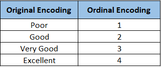
 

Categorical data encoding - ordinal encoding
An example of ordinal encoding – Source: Medium


How Ordinal Encoding Works

Ordinal encoding involves mapping each category to a unique integer value that reflects the order of the categories. This method ensures that the encoded values preserve the inherent order among the categories. It can be summed into the following steps

  1. Determine the ordinal feature in your dataset that needs to be encoded.
  2. Establish a meaningful order for the categories.
  3. Assign a unique integer to each category based on their order.
  4. Replace the original categories in the feature with their corresponding integer values.

Advantages of Ordinal Encoding

  1. Preserves Order: It captures and preserves the ordinal relationships between categories, which can be valuable for certain types of analyses.
  2. Reduces Dimensionality: It reduces the dimensionality of the dataset compared to one-hot encoding, making it more memory-efficient.
  3. Compatible with Many Algorithms: It provides a numerical representation of the data, making it suitable for many machine learning algorithms.

Use Cases

  1. Ordinal Data: When dealing with categorical features that exhibit a clear and meaningful order or ranking. For example, education levels, satisfaction ratings, or any other feature with an inherent order.
  2. Machine Learning Models: Algorithms like linear regression, decision trees, and support vector machines can benefit from the ordered numerical representation of ordinal features.

Challenges with Ordinal Encoding

  1. Assumption of Linear Relationships: Some machine learning algorithms might assume a linear relationship between the encoded integers, which might not always be appropriate for all ordinal features.
  2. Not Suitable for Nominal Data: It should not be applied to nominal categorical features, where the categories do not have a meaningful order.

Ordinal encoding is especially useful for machine learning algorithms that need numerical input and can handle the ordered nature of the data.


How generative AI and LLMs work


6. Count Encoding

Count encoding, also known as frequency encoding, is a technique used to convert categorical features into numerical values based on the frequency of each category in the dataset.

This method assigns each category a numerical value representing how often it appears, thereby providing a straightforward numerical representation of the categories.


Categorical data encoding - count encoding
An example of count encoding – Source: Medium


How Count Encoding Works

The process of count encoding involves mapping each category to its frequency or count within the dataset. Categories that appear more frequently receive higher values, while less common categories receive lower values. This can be particularly useful in scenarios where the frequency of categories carries significant information.

  1. Determine the categorical feature in your dataset that needs to be encoded.
  2. Calculate the frequency of each category within the feature.
  3. Assign the calculated frequencies as numerical values to each corresponding category.
  4. Replace the original categories in the feature with their corresponding frequency values.

Advantages of Count Encoding

  1. Simple and Interpretable: It provides a straightforward and interpretable way to encode categorical data, preserving the count information.
  2. Relevant for Frequency-Based Problems: Particularly useful when the frequency of categories is a relevant feature for the problem you’re solving.
  3. Reduces Dimensionality: It reduces the dimensionality compared to one-hot encoding, which can be beneficial in high-cardinality scenarios.

Use Cases

  1. Frequency-Relevant Features: When analyzing categorical features where the frequency of each category is relevant information for your model. For instance, in customer segmentation, the frequency of customer purchases might be crucial.
  2. High-Cardinality Features: When dealing with high-cardinality categorical features, where one-hot encoding would result in a large number of columns, count encoding provides a more compact representation.

Challenges with Count Encoding

  1. Loss of Category Information: It can lose some information about the distinctiveness of categories since categories with the same frequency will have the same encoded value.
  2. Not Suitable for Ordinal Data: It should not be applied to ordinal categorical features where the order of categories is important.

Count encoding is a valuable technique for scenarios where category frequencies carry significant information and when dealing with high-cardinality features.

7. Binary Encoding

Binary encoding is a versatile technique for encoding categorical features, especially when dealing with high-cardinality data. It combines the benefits of one-hot and label encoding while reducing dimensionality.
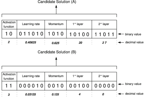
 

Categorical data encoding - binary encoding
An example of binary encoding – Source: ResearchGate


How Binary Encoding Works

Binary encoding involves converting each category into binary code and representing it as a sequence of binary digits (0s and 1s). Each binary digit is then placed in a separate column, effectively creating a set of binary columns for each category. The encoding process follows these steps:

  1. Assign a unique integer to each category, similar to label encoding.
  2. Convert the integer to binary code.
  3. Create a set of binary columns to represent the binary code.

Advantages of Binary Encoding

  1. Dimensionality Reduction: It reduces the dimensionality compared to one-hot encoding, especially for features with many unique categories.
  2. Memory Efficient: It is memory-efficient and overcomes the curse of dimensionality.
  3. Easy to Implement and Interpret: It is straightforward to implement and interpret.

Use Cases

  1. High-Cardinality Features: When dealing with high-cardinality categorical features (features with a large number of unique categories), binary encoding helps reduce the dimensionality of the dataset.
  2. Machine Learning Models: It is suitable for many machine learning algorithms that can handle binary input features effectively.

Challenges with Binary Encoding

  1. Complexity: Although binary encoding reduces dimensionality, it might still introduce complexity for features with extremely high cardinality.
  2. Handling Missing Values: Special care is needed to handle missing values during the encoding process.

Hence, binary encoding combines the advantages of one-hot encoding and label encoding, making it a suitable choice for many ML tasks.


Mastering Categorical Data Encoding for Enhanced Machine Learning

In summary, the effective handling of categorical data is a cornerstone of modern machine learning. With the growth of machine learning models, businesses can now manage data more efficiently, leading to improved enterprise performance.

This blog has delved into the basics of categorical data and outlined seven critical encoding methods. Each method has its unique advantages, challenges, and specific use cases, making it essential to choose the right technique based on the nature of the data and the requirements of the model.


Explore a hands-on curriculum that helps you build custom LLM applications!


Proper encoding not only ensures compatibility with various models but also enhances pattern recognition, prevents bias, and improves feature engineering. By mastering these encoding techniques, data scientists can significantly improve model performance and make more informed predictions, ultimately driving better business outcomes.


You can also join our Discord community to stay posted and participate in discussions around machine learning, AI, LLMs, and much more!

What is Categorical Data Encoding? 7 Effective Methods | Data Science Dojo

July 23, 2024

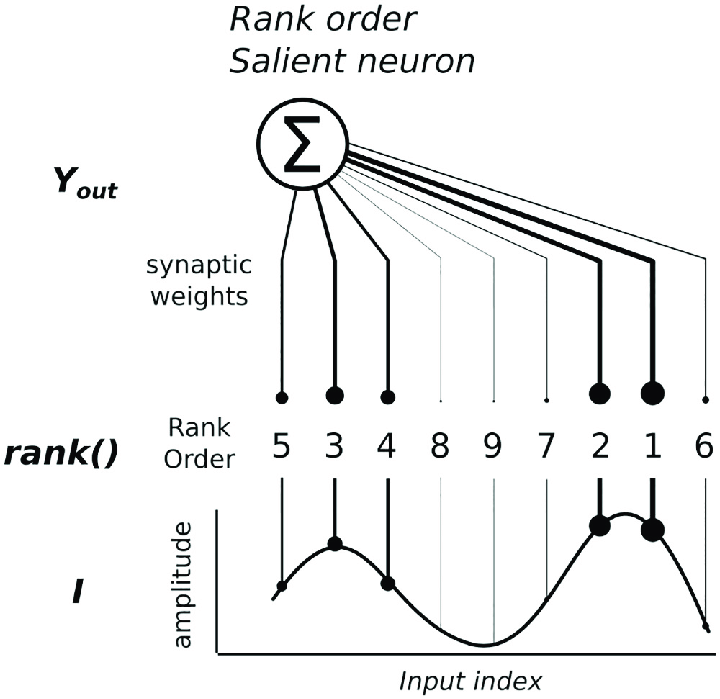
In this blog, we’re diving into a new approach called rank-based encoding that promises not just to shake things up but to guarantee top-notch results.


Rank-based encoding – a breakthrough?


Say hello to rank-based encoding – a technique you probably haven’t heard much about yet, but one that’s about to change the game.


rank-based encoding
An example illustrating rank-based encoding – Source: ResearchGate


In the vast world of machine learning, getting your data ready is like laying the groundwork for success. One key step in this process is encoding – a way of turning non-numeric information into something our machine models can understand. This is particularly important for categorical features – data that is not in numbers.


Join us as we explore the tricky parts of dealing with non-numeric features, and how rank-based encoding steps in as a unique and effective solution. Get ready for a breakthrough that could redefine your machine-learning adventures – making them not just smoother but significantly more impactful.


Problem under consideration


In our blog, we’re utilizing a dataset focused on House Price Prediction to illustrate various encoding techniques with examples. In this context, we’re treating the city categorical feature as our input, while the output feature is represented by the price.


Large language model bootcamp


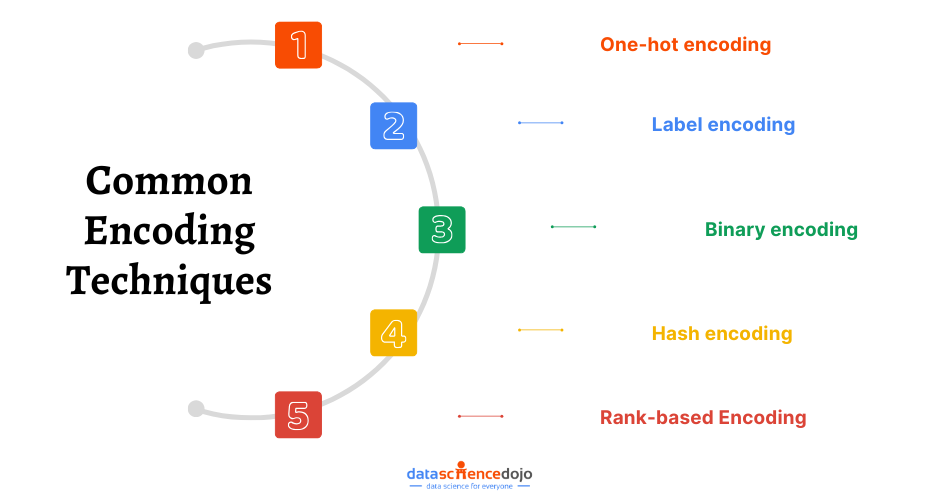
Some common techniques


The following section will cover some of the commonly used techniques and their challenges. We will conclude by digging deeper into rank-based encoding and how it overcomes these challenges.


  • One-hot encoding  


In One-hot encoding, each category value is represented as an n-dimensional, sparse vector with zero entries except for one of the dimensions. For example, if there are three values for the categorical feature City, i.e. Chicago, Boston, Washington DC, the one-hot encoded version of the city will be as depicted in Table 1.


If there is a wide range of categories present in a categorical feature, one-hot encoding increases the number of columns(features) linearly which requires high computational power during the training phase.  


City  City Chicago  City Boston  Washington DC 
Chicago  1  0  0 
Boston  0  1  0 
Washington DC  0  0  1 

  Table 1 


  • Label encoding  


This technique assigns a label to each value of a categorical column based on alphabetical order. For example, if there are three values for the categorical feature City, i.e. Chicago, Boston, Washington DC, the label encoded version will be as depicted in Table 2.


Since B comes first in alphabetical order, this technique assigns Boston the label 0, which leads to meaningless learning of parameters.  


City  City Label Encoding 
Chicago  1 
Boston  0 
Washington DC  2 

Table 2 


  • Binary encoding  


It involves converting each category into a binary code and then splitting the resulting binary string into columns. For example, if there are three values for the categorical feature City, i.e. Chicago, Boston, Washington DC, the binary encoded version of a city can be observed from Table 3.


Since there are 3 cities, two bits would be enough to uniquely represent each category. Therefore, two columns will be constructed which increases dimensions. However, this is not meaningful learning as we are assigning more weightage to one category than others.


Chicago is assigned 00, so our model would give it less weightage during the learning phase. If any categorical column has a wide range of unique values, this technique requires a large amount of computational power, as an increase in the number of bits results in an increase in the number of dimensions (features) significantly. 


City  City 0  City 1 
Chicago  0  0 
Boston  0  1 
Washington DC  1  0 

  Table 3 


  • Hash encoding  


It uses the hashing function to convert category data into numerical values. Using hashed functions solves the problem of a high number of columns if the categorical feature has a large number of categories. We can define how many numerical columns we want to encode our feature into.


However, in the case of high cardinality of a categorical feature, while mapping it into a lower number of numerical columns, loss of information is inevitable. If we use a hash function with one-to-one mapping, the result would be the same as one-hot encoding. 


  • Rank-based Encoding: 


In this blog, we propose rank-based encoding which aims to encode the data in a meaningful manner with no increase in dimensions. Thus, eliminating the increased computational complexity of the algorithm as well as preserving all the information of the feature.


Rank-based encoding works by computing the average of the target variable against each category of the feature under consideration. This average is then sorted in decreasing order from high to low and each category is assigned a rank based on the corresponding average of a target variable. An example is illustrated in Table 4 which is explained below:


The average price of Washington DC = (60 + 55)/2 = 57.5 Million 

The average price of Boston = (20 +12+18)/3 = 16.666 Million 

The average price of Chicago = (40 + 35)/2 = 37.5 Million


In the rank-based encoding process, each average value is assigned a rank in descending order.


For instance, Washington DC is given rank 1, Chicago gets rank 2, and Boston is assigned rank 3. This technique significantly enhances the correlation between the city (input feature) and price variable (output feature), ensuring more efficient model learning.


Learn to build LLM applications


In my evaluation, I assessed model metrics such as R2 and RMSE. The results demonstrated significantly lower values compared to other techniques discussed earlier, affirming the effectiveness of this approach in improving overall model performance. 


City  Price  City Rank 
Washington DC  60 Million  1 
Boston  20 Million  3 
Chicago  40 Million  2 
Chicago  35 Million  2 
Boston  12 Million  3 
Washington DC  55 Million  1 
Boston  18 Million  3 

Table 4 


Results


We summarize the pros and cons of each technique in Table 5. Rank-based encoding emerges to be the best in all aspects. Effective data preprocessing is crucial for the optimal performance of machine learning models. Among the various techniques, rank-based encoding is a powerful method that contributes to enhanced model learning.


Rank-based encoding technique facilitates a stronger correlation between input and output variables, leading to improved model performance. The positive impact is evident when evaluating the model using metrics like RMSE and R2 etc. In our case, these enhancements reflect a notable boost in overall model performance. 


Encoding Technique  Meaningful Learning  Loss of Information  Increase in Dimensionality 
One-hot x 
Label x  x 
Binary x  x 
Hash x 
Rank-based x  x 

Table 5 

February 2, 2024

Transformers have revolutionized natural language processing with their use of self-attention mechanisms. In this post, we will study the key components of transformers to understand how they have become the basis of the state of the art in different tasks.  


Introduction: Attention is all you need 

The Transformer architecture was first introduced in the 2017 paper “Attention is All You Need” by researchers at Google. Unlike previous sequence models such as RNNs, Transformer relies entirely on self-attention to model dependencies in sequential data like text.   


Large language models knowledge test


Remarkably, this simple change led to major improvements in machine translation quality over existing methods. Since then, Transformers have been applied successfully to diverse NLP tasks like text generation, summarization, and question-answering. Their versatility has even led to applications in computer vision 


Large language model bootcamp


But what exactly is self-attention and why is it so effective? Let’s explore this. 

The limitations of Recurrent Neural Networks – RNNs   

Recurrent neural networks (RNNs) used to be the dominant approach for modeling sequences. An RNN processes textual data incrementally, maintaining a “memory” of the previous context. For example, to predict the next word in a sentence, an RNN model would incorporate information about all the preceding words.  

However, RNNs have certain limitations. They process data sequentially, making parallelization difficult. More critically, they struggle to learn long-range dependencies because the information gets diluted over many steps of time. Attention mechanisms were proposed to mitigate this issue. 

Learn to build LLM applications

Why use a transformer model?  

The transformer architecture has enabled the development of new models that can be trained on large datasets and significantly outperform recurrent neural networks like LSTMs. These new models are utilized for tasks like sequence classification, question answering, language modeling, named entity recognition, summarization, and translation.  

Let’s examine the key components of transformers to understand how they have become the foundation for state-of-the-art performance on different NLP tasks.  

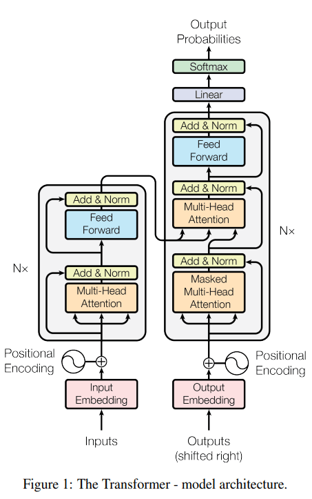
Transformer design  

A transformer consists of an encoder and a decoder. The encoder’s role is to encode the inputs (i.e. sentences) into a state, often containing multiple tensors. This state is then passed to the decoder to generate the outputs.

In machine translation, the encoder converts a source sentence, e.g. “Hello world“, into a state, such as a vector, that captures its semantic meaning.

The decoder then utilizes this state to produce the translated target sentence, e.g. “Bonjour le monde.” Both the encoder and decoder primarily employ Multi-Head Attention and Feedforward Networks, which are the focus of this article.   


Transformer model architecture

Key transformer components  

1. Input embedding  

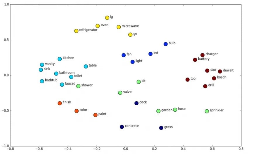
Embedding aims to create a vector representation of words where words with similar meanings will be close in terms of Euclidean distance. For instance, the words “bathroom” and “shower” are related to the same concept, so their word vectors are close in Euclidean space as they convey similar meanings.  

For the encoder, the authors opted for an embedding size of 512 (i.e. each word is represented by a 512-dimensional vector).  


  Input embedding


2. Positional encoding  

The position of a word plays a crucial role in understanding the sequence we want to model.  

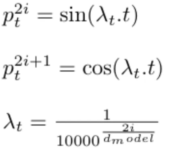
Therefore, we add positional information about the word’s location in the sequence to its vector. The authors used the following sinusoidal. 

Position encoding   


We will explain positional encoding in more detail with an example.  

  Position encoding example


We note the position of each word in the sequence.  

We define dmodel = 512, which represents the size of the embedding vector of each word (i.e. the vector dimension). We can now rewrite the two positional encoding equations as:  


two positional encoding equations


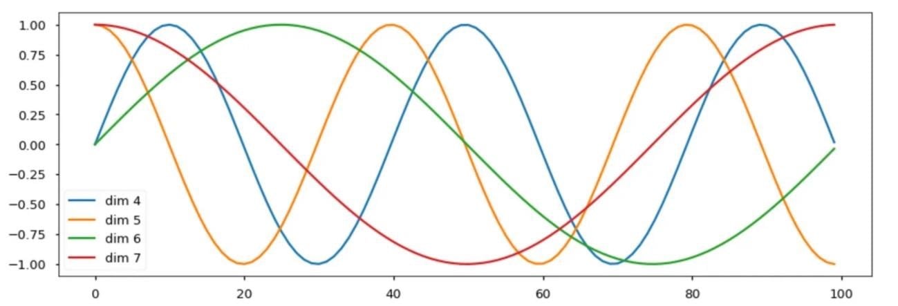
We can see that the wavelength (i.e. frequency) λt decreases as the dimension increases, this forms a progression along the wave from 2pi to 10000.2pi.  


  wavelength


In this model, the absolute positional information of a word in a sequence is added directly to its initial vector. For this, the positional encoding must have the same size dmodel as the initial word vector.  


3.
Attention mechanism  

  • Scaled Dot-Product Attention  

  Scaled Dot-Product Attention


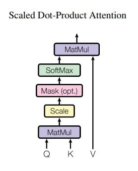
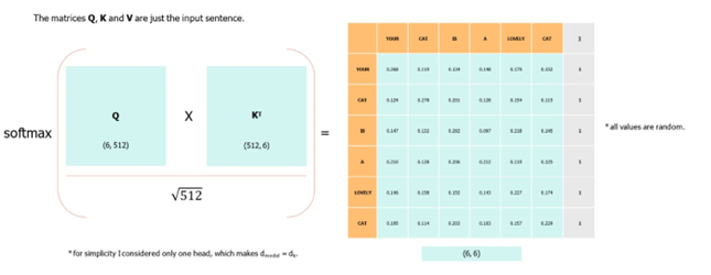
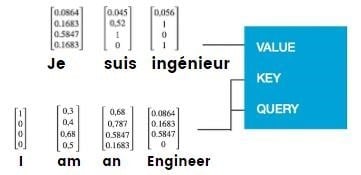
Let’s explain the attention mechanism. The key goal of attention is to estimate the relative relevance of the keywords compared to the query word for the same entity. For this, the attention mechanism takes a query vector Q representing a word, the keys K comprising all other words in the sentence, and values V representing the word vectors.  

In our case, V = Q (for the two self-attention layers). In other words, the attention mechanism provides the significance of a word in a given sentence.  


attention mechanism


When we compute the normalized dot product between the query and the keys, we get a tensor that represents the relative importance of each other word for the query. To go deeper into mathematics, we can try to understand why the authors used a dot product to calculate the relation between two words.  


Get Started with Generative AI                                    


A word is represented by a vector in Euclidian space, in this case, a vector of size 512.   

When computing the dot product between Q and KT, we calculate the product between Q’s orthogonal projection onto K. In other words, we estimate the alignment between the query and keyword vectors, returning a weight for each word in the sentence.  

We then normalize by dk to counteract large Q and K magnitudes which can push the softmax function into regions with tiny gradients. The softmax function regularizes the terms and rescales them between 0 and 1 (i.e., converts the dot product to a probability distribution), with the goal of normalizing all weights between 0 and 1.  

  softmax function

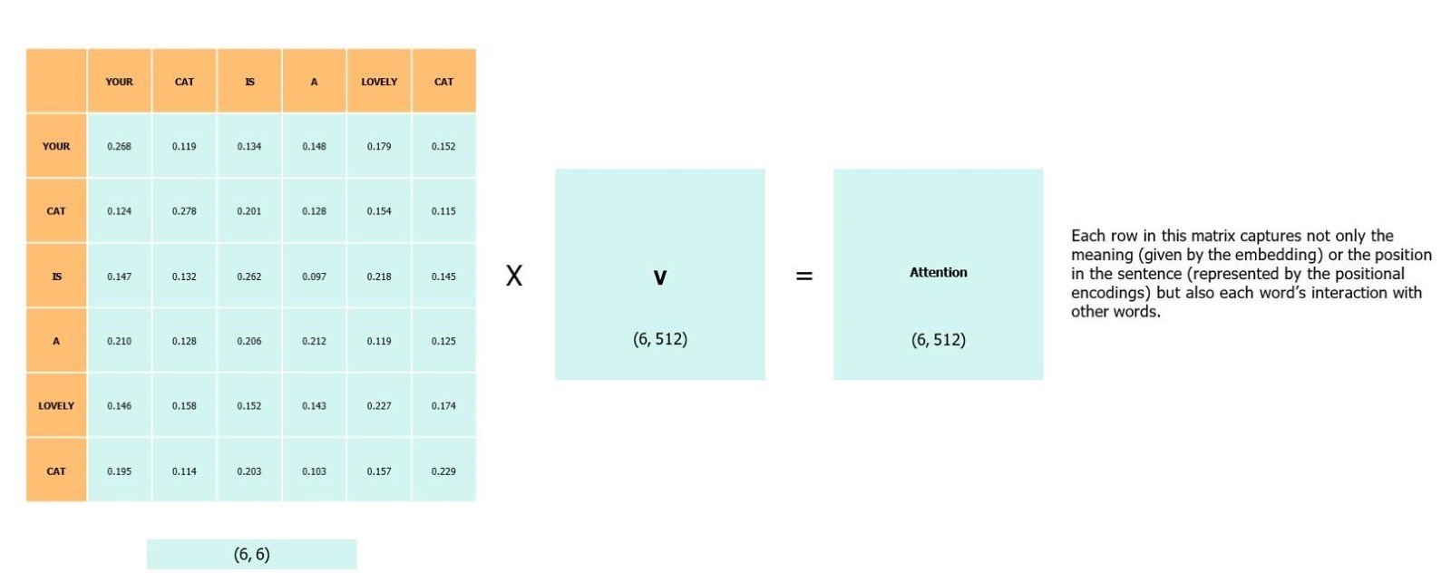
Finally, we multiply the weights (i.e., importance) by the values V to reduce irrelevant words and focus on the most significant words.  


Attention mechanism (2)


  • Multi-Head Attention  

  Multi-Head Attention


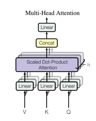
The key idea is that attention is applied multiple times in parallel on different projections of the input queries, keys, and values. This allows the model to learn different types of dependencies between the input words.  


The input queries (Q), keys (K), and values (V) are each linearly projected h times into smaller subspaces. For example, h=8 times into 64-dimensional spaces.  

Attention is then applied in each of these h projected subspaces in parallel, yielding h different attention outputs.  


Attention mechanism and transformers - LLM
Attention mechanism and transformers – LLM Bootcamp Data Science Dojo


These h outputs are concatenated and linearly projected again to get the final values. The projections allow the model to focus on different positional and semantic relationships between words since each projected subspace captures different information.  

Doing this in parallel (multi-head) instead of sequentially improves efficiency.  

The projection matrices are learned during training to discover the most useful projections. So, in summary, multi-head attention applies the attention mechanism in multiple parallel subspaces to learn different types of dependencies between words in an efficient way.  


Let’s dive into the mechanics of encoder-decoder architecture.  

Transformer model architecture   


In this section, we’ll explain how the encoder and decoder work together to translate an English sentence into a French one, step by step.  

1. Encoder  

Encoder

  • Convert a sequence of tokens to a sequence of vectors by using embeddings.    

Positional encoding


  • Add position information in each word vector.  


The key advantage of recurrent neural networks is their knack for understanding relationships between sequences and remembering information. On the other hand, Transformers employ positional encoding to factor in where words are in a sequence.  

  • Apply Multi-Head Attention  

Apply Multi-Head Attention   

  • Use Feed Forward Network  


2. Decoder  

  • Utilize embeddings to transform a French sentence into vectors.   

  decoder French


  • Add positional details within each word vector.    

Positional encoding French   

  • Apply Multi-Head Attention  

  Apply Multi-Head Attention French


  • Apply Feed Forward Network  


  • Apply Multi-Head Attention to the encoder output.  

Multi-Head Attention - encoder output
 

We can observe that the Transformer combines the encoder’s output with the decoder’s input. This enables it to discern the relationship between the vectors that encode the English and French sentences.  

  • Apply the Feed Forward Network again.  
  • Compute the probability for the next word by using linear + SoftMax block. The decoder returns the highest probability as the next word at the output.  

  Linear and SoftMax block

In our case, the next word after “Je” is “suis” 


Final thoughts 

The transformer model outperforms all the models on different benchmarks also there was no difference seen between the translation provided by the algorithm and by humans.   

Transformers are a major advance in NLP, they exceed RNN by having a lower training cost allowing to train models on larger corpora. Even today, transformers remain the basis of state-of-the-art models such as BERT, Roberta, XLNET, and GPT.  


References: 

https://proceedings.neurips.cc/paper_files/paper/2017/file/3f5ee243547dee91fbd053c1c4a845aa-Paper.pdf 

https://github.com/hkproj/transformer-from-scratch-notes 

http://jalammar.github.io/illustrated-transformer/ 

October 18, 2023

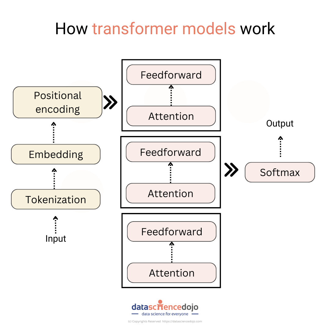
Transformer models are a type of deep learning model that is used for natural language processing (NLP) tasks. They can learn long-range dependencies between words in a sentence, which makes them very powerful for tasks such as machine translation, text summarization, and question answering.

Transformer models work by first encoding the input sentence into a sequence of vectors. This encoding is done using a self-attention mechanism, which allows the model to learn the relationships between the words in the sentence.

Once the input sentence has been encoded, the model decodes it into a sequence of output tokens. This decoding is also done using a self-attention mechanism.

The attention mechanism is what allows transformer models to learn long-range dependencies between words in a sentence. The attention mechanism works by focusing on the most relevant words in the input sentence when decoding the output tokens.

Learn in detail about transformer models here:

Large language model bootcamp

Transformer models are very powerful, but they can be computationally expensive to train. However, they are constantly being improved, and they are becoming more efficient and powerful all the time.

History

The history of transformers in neural networks can be traced back to the early 1990s when Jürgen Schmidhuber proposed the first transformer model. This model was called the “fast weight controller” and it used a self-attention mechanism to learn the relationships between words in a sentence. However, the fast-weight controller was not very efficient, and it was not widely used.

In 2017, Vaswani et al. published the paper “Attention is All You Need”, which introduced a new transformer model that was much more efficient than the fast-weight controller. This new model, which is now simply called the “transformer”, quickly became state-of-the-art for a wide range of natural language efficient (NLP) tasks, including machine translation, text summarization, and question answering.

Learn more about NLP in this blog —-> Applications of Natural Language Processing

The transformer has been so successful because it can learn long-range dependencies between words in a sentence. This is essential for many NLP tasks, as it allows the model to understand the context of a word in a sentence. The transformer does this using a self-attention mechanism, which allows the model to focus on the most relevant words in a sentence when decoding the output tokens.

The transformer has had a major impact on the field of NLP. It is now the go-to approach for many NLP tasks, and it is constantly being improved. In the future, transformers are likely to be used to solve a wider range of NLP tasks, and they will become even more efficient and powerful.

Here are some of the key events in the history of transformers in neural networks:

  • 1990: Jürgen Schmidhuber proposes the first transformer model, the “fast weight controller”.
  • 2017: Vaswani et al. publish the paper “Attention is All You Need”, which introduces the transformer model.
  • 2018: Transformer models achieve state-of-the-art results on a wide range of NLP tasks, including machine translation, text summarization, and question answering.
  • 2019: Transformers are used to create large language models (LLMs) such as BERT and GPT-2.
  • 2020: LLMs are used to create even more powerful models such as GPT-3.

The history of transformers in neural networks is still being written. It is an exciting time to be in the field of NLP, as transformers are making it possible to solve previously intractable problems.


NLP transformer architecture

The transformer model is made up of two main components: an encoder and a decoder. The encoder takes the input sentence as input and produces a sequence of vectors. The decoder then takes these vectors as input and produces the output sentence.

transformer models
How a transfer model works

The encoder consists of a stack of self-attention layers. Each self-attention layer takes a sequence of vectors as input and produces a new sequence of vectors. The self-attention layer works by first computing a score for each pair of words in the input sequence. The score for a pair of words is a measure of how related the two words are. The self-attention layer then uses these scores to compute a weighted sum of the input vectors. The weighted sum is the output of the self-attention layer.

The decoder consists of a stack of self-attention layers and a recurrent neural network (RNN). The self-attention layers work the same way as in the encoder. The RNN takes the output of the self-attention layers as input and produces a sequence of output tokens. The output tokens are the words in the output sentence.

The attention mechanism is what allows the transformer model to learn long-range dependencies between words in a sentence. The attention mechanism works by focusing on the most relevant words in the input sentence when decoding the output tokens.

For example, let’s say we want to translate the sentence “I love you” from English to Spanish. The transformer model would first encode the sentence into a sequence of vectors. Then, the model would decode the vectors into a sequence of Spanish words. The attention mechanism would allow the model to focus on the words “I” and “you” in the English sentence when decoding the Spanish words “te amo”.

Transformer models are a powerful tool for NLP, and they are constantly being improved. They are now the go-to approach for many NLP tasks, and they are constantly being improved.

Learn More                  

Encoding and Decoding

Encoding and decoding are two key concepts in natural language processing (NLP). Encoding is the process of converting a sequence of words into a sequence of vectors. Decoding is the process of converting a sequence of vectors back into a sequence of words.

Encoding

The encoder in a transformer model takes a sequence of words as input and produces a sequence of vectors. The encoder consists of a stack of self-attention layers. Each self-attention layer takes a sequence of vectors as input and produces a new sequence of vectors. The self-attention layer works by first computing a score for each pair of words in the input sequence. The score for a pair of words is a measure of how related the two words are. The self-attention layer then uses these scores to compute a weighted sum of the input vectors. The weighted sum is the output of the self-attention layer.

For example, let’s say we have the sentence “I like you”. The encoder would first compute a score for each pair of words in the sentence. The score for the word “I” and the word “like” would be high, because these words are related. The score for the word “like” and the word “you” would also be high, for the same reason. The encoder would then use these scores to compute a weighted sum of the input vectors. The weighted sum would be a vector that represents the meaning of the sentence “I like you”.

Decoding

The decoder in a transformer model takes a sequence of vectors as input and produces a sequence of words. The decoder also consists of a stack of self-attention layers. The self-attention layers work the same way as in the encoder. The decoder also has an RNN, which takes the output of the self-attention layers as input and produces a sequence of output tokens. The output tokens are the words in the output sentence.

For example, let’s say we want to translate the sentence “I love you” from English to Spanish. The decoder would first take the vector that represents the meaning of the sentence “I love you” as input. Then, the decoder would use the self-attention layers to compute a weighted sum of the input vectors. The weighted sum would be a vector that represents the meaning of the sentence “I love you” in Spanish. The decoder would then use the RNN to produce a sequence of Spanish words. The output of the RNN would be the Spanish sentence “Te amo”

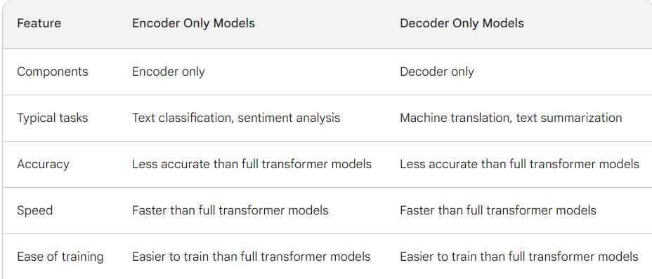
Encoder only models

Encoder-only models are a type of transformer model that only has an encoder. Encoder-only models are typically used for tasks like text classification, where the model only needs to understand the meaning of the input text.

For example, an encoder-only model could be used to classify a news article as either “positive” or “negative”. The encoder would first encode the article into a sequence of vectors. Then, the model would use a classifier to classify the article.

Encoder-only models are typically less powerful than full transformer models, but they are much faster and easier to train. This makes them a good choice for tasks where speed and efficiency are more important than accuracy.

Decoder only models

Decoder-only models are a type of transformer model that only has a decoder. Decoder-only models are typically used for tasks like machine translation, where the model needs to generate the output text.

For example, a decoder-only model could be used to translate a sentence from English to Spanish. The decoder would first take the English sentence as input. Then, the decoder would use the self-attention layers to compute a weighted sum of the input vectors. The weighted sum would be a vector that represents the meaning of the sentence in Spanish. The decoder would then use an RNN to produce a sequence of Spanish words. The output of the RNN would be the Spanish sentence.

Decoder-only models are typically less powerful than full transformer models, but they are much faster and easier to train. This makes them a good choice for tasks where speed and efficiency are more important than accuracy.

Here is a table that summarizes the differences between encoder-only models and decoder-only models:

Differences between a decoder-only and an encoder-only transformer model

What are transformer models built of

Transformer models are built of the following components:

  • Embedding layer: The embedding layer converts the input text into a sequence of vectors. The vectors represent the meaning of the words in the text.
  • Self-attention layers: The self-attention layers allow the model to learn long-range dependencies between words in a sentence. The self-attention layers work by computing a score for each pair of words in the sentence. The score for a pair of words is a measure of how related the two words are. The self-attention layers then use these scores to compute a weighted sum of the input vectors. The weighted sum is the output of the self-attention layer.
  • Positional encoding: The positional encoding layer adds information about the position of each word in the sentence. This is important for learning long-range dependencies, as it allows the model to know which words are close to each other in the sentence.
  • Decoder: The decoder takes the output of the self-attention layers as input and produces a sequence of output tokens. The output tokens are the words in the output sentence.

Transformer models are also typically trained with the following techniques:

  • Masked language modeling: Masked language modeling is a technique used to train transformer models to predict the missing words in a sentence. This helps the model to learn to attend to the most relevant words in a sentence.
  • Attention masking: Attention masking is a technique used to prevent the model from attending to future words in a sentence. This is important for preventing the model from learning circular dependencies.
  • Gradient clipping: Gradient clipping is a technique used to prevent the gradients from becoming too large. This helps to stabilize the training process and prevent the model from overfitting.

Attention layers are a type of neural network layer that allows the model to learn long-range dependencies between words in a sentence. The attention layer works by computing a score for each pair of words in the sentence. The score for a pair of words is a measure of how related the two words are. The attention layer then uses these scores to compute a weighted sum of the input vectors. The weighted sum is the output of the attention layer.

The input to the attention layer is a sequence of vectors. The output of the attention layer is a weighted sum of the input vectors. The weights are computed using the scores for each pair of words in the sentence.

The attention layer can learn long-range dependencies because it allows the model to attend to any word in the sentence, regardless of its position. This is in contrast to recurrent neural networks (RNNs), which can only attend to words that are close to the current word.

Transformer architecture is a neural network architecture that is based on attention layers. Transformer models are typically made up of an encoder and a decoder. The encoder takes the input text as input and produces a sequence of vectors. The decoder takes the output of the encoder as input and produces a sequence of output tokens.

The encoder consists of a stack of self-attention layers. The decoder also consists of a stack of self-attention layers. The self-attention layers in the decoder can attend to both the input text and the output text. This allows the decoder to generate the output text in a way that is consistent with the input text.

Transformer models are typically trained with the masked language modeling technique. Masked language modeling is a technique used to train transformer models to predict the missing words in a sentence. This helps the model to learn to attend to the most relevant words in a sentence.

Tackle transformer model challenges

Transformer models are a powerful tool for natural language processing (NLP) tasks, but they can be challenging to train and deploy. Here are some of the challenges of transformer models and how to tackle them:
  • Computational complexity: Transformer models are very computationally expensive to train and deploy. This is because they require a large number of parameters and a lot of data. To tackle this challenge, researchers are developing new techniques to make transformer models more efficient.
  • Data requirements: Transformer models require a large amount of data to train. This is because they need to learn the relationships between words in a sentence. To tackle this challenge, researchers are developing new techniques to pre-train transformer models on large datasets.
  • Interpretability: Transformer models are not as interpretable as other machine learning models, such as decision trees and logistic regression. This makes it difficult to understand why the model makes the predictions that it does. To tackle this challenge, researchers are developing new techniques to make transformer models more interpretable.

Here are some specific techniques that have been developed to tackle the challenges of transformer models:

  • Knowledge distillation: Knowledge distillation is a technique that can be used to train a smaller, more efficient transformer model by distilling the knowledge from a larger, more complex transformer model.
  • Data augmentation: Data augmentation is a technique that can be used to increase the size of a dataset by creating new data points from existing data points. This can help to improve the performance of transformer models on small datasets.
  • Attention masking: Attention masking is a technique that can be used to prevent the transformer model from attending to future words in a sentence. This helps to prevent the model from learning circular dependencies.
  • Gradient clipping: Gradient clipping is a technique that can be used to prevent the gradients from becoming too large. This helps to stabilize the training process and prevent the model from overfitting.
August 16, 2023

Related Topics

Statistics
Resources
rag
Programming
Machine Learning
LLM
Generative AI
Data Visualization
Data Security
Data Science
Data Engineering
Data Analytics
Computer Vision