R

SQL (Structured Query Language) is an important tool for data scientists. It is a programming language used to manipulate data stored in relational databases. Mastering SQL concepts allows a data scientist to quickly analyze large amounts of data and make decisions based on their findings. Here are some essential SQL concepts that every data scientist should know:

First, understanding the syntax of SQL statements is essential in order to retrieve, modify or delete information from databases. For example, statements like SELECT and WHERE can be used to identify specific columns and rows within the database that need attention. A good knowledge of these commands can help a data scientist perform complex operations with ease.

Second, developing an understanding of database relationships such as one-to-one or many-to-many is also important for a data scientist working with SQL.

Here’s an interesting read about Top 10 SQL commands

Let’s dive into some of the key SQL concepts that are important to learn for a data scientist.  

1. Formatting Strings

We are all aware that cleaning up the raw data is necessary to improve productivity overall and produce high-quality decisions. In this case, string formatting is crucial and entails editing the strings to remove superfluous information. For transforming and manipulating strings, SQL provides a large variety of string methods. When combining two or more strings, CONCAT is utilized. The user-defined values that are frequently required in data science can be substituted for the null values using COALESCE. Tiffany Payne  

2. Stored Methods

We can save several SQL statements in our database for later use thanks to stored procedures. When invoked, it allows for reusability and has the ability to accept argument values. It improves performance and makes modifications simpler to implement. For instance, we’re attempting to identify all A-graded students with majors in data science. Keep in mind that CREATE PROCEDURE must be invoked using EXEC in order to be executed, exactly like the function definition. Paul Somerville 

3. Joins

Based on the logical relationship between the tables, SQL joins are used to merge the rows from various tables. In an inner join, only the rows from both tables that satisfy the specified criteria are displayed. In terms of vocabulary, it can be described as an intersection. The list of pupils who have signed up for sports is returned. Sports ID and Student registration ID are identical, please take note. Left Join returns every record from the LEFT table, while Right Join only shows the matching entries from the RIGHT table. Hamza Usmani 

4. Subqueries

Knowing how to utilize subqueries is crucial for data scientists because they frequently work with several tables and can use the results of one query to further limit the data in the primary query. The nested or inner query is another name for it. The subquery is conducted before the main query and needs to be surrounded in parenthesis. It is referred to as a multi-line subquery and requires the use of multi-line operators if it returns more than one row. Tiffany Payne 

5. Left Joins vs Inner Joins

It’s easy to confuse left joins and inner joins, especially for those who are still getting their feet wet with SQL or haven’t touched the language in a while. Make sure that you have a complete understanding of how the various joins produce unique outputs. You will likely be asked to do some kind of join in a significant number of interview questions, and in certain instances, the difference between a correct response and an incorrect one will depend on which option you pick. Tom Miller 

6. Manipulation of dates and times

There will most likely be some kind of SQL query using date-time data, and you should prepare for it. For instance, one of your tasks can be to organize the data into groups according to the months or to change the format of a variable from DD-MM-YYYY to only the month. You should be familiar with the following functions:

– EXTRACT
– DATEDIFF
– DATE ADD, DATE SUB
– DATE TRUNC 

Olivia Tonks 

7. Procedural Data Storage 

Using stored procedures, we can compile a series of SQL commands into a single object in the database and call it whenever we need it. It allows for reusability and when invoked, can take in values for its parameters. It improves efficiency and makes it simple to implement new features. Using this method, we can identify the students with the highest GPAs who have declared a particular major. One goal is to identify all A-students whose major is Data Science. It’s important to remember that, like a function declaration, calling a CREATE PROCEDURE with EXEC is necessary for the procedure to be executed. Nely Mihaylova 

8. Connecting SQL to Python or R 

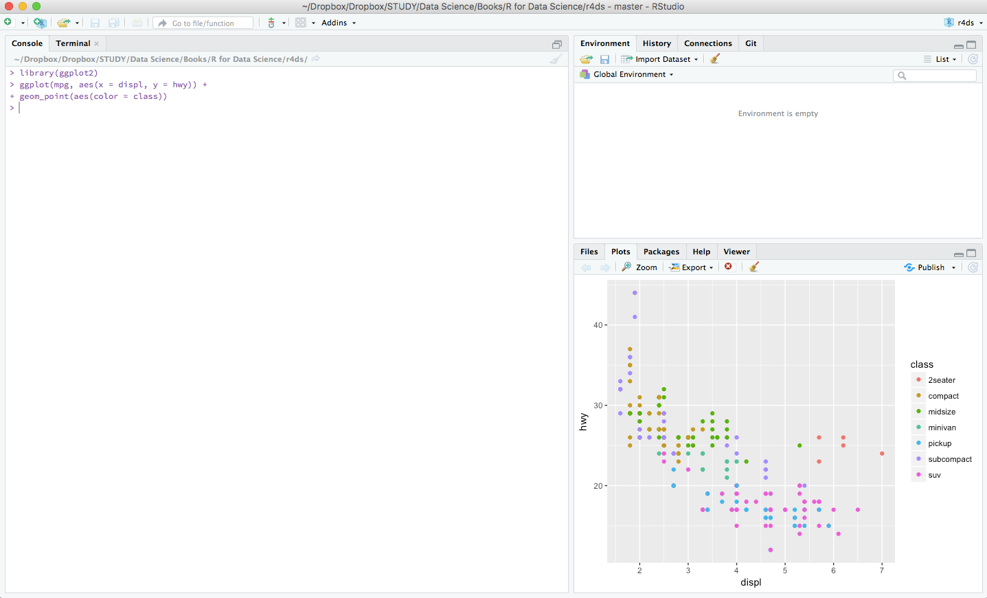
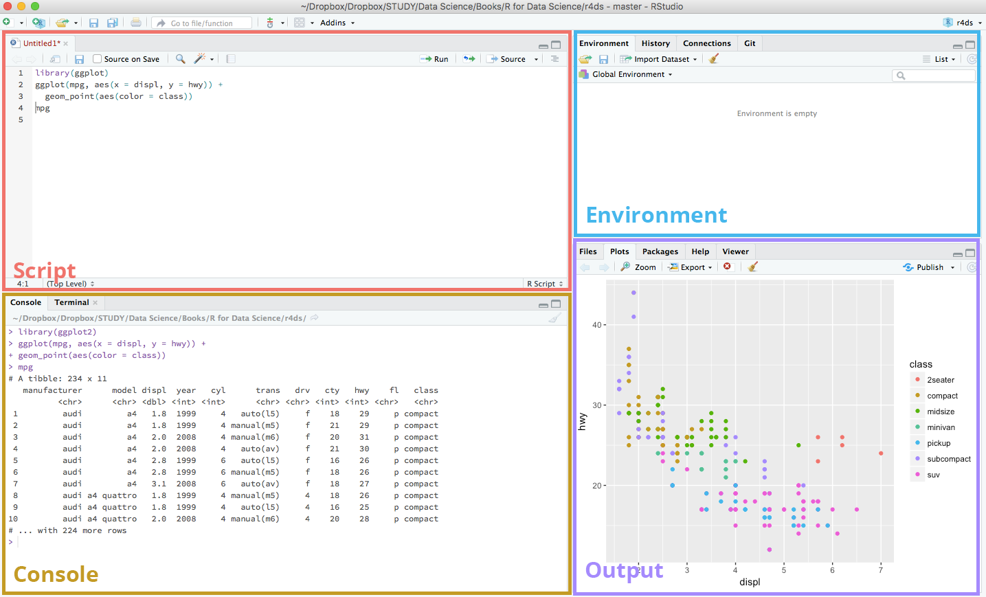
A developer who is fluent in a statistical language, like Python or R, may quickly and easily use the packages of
language to construct machine learning models on a massive dataset stored in a relational database management system. A programmer’s employment prospects will improve dramatically if they are fluent in both these statistical languages and SQL. Data analysis, dataset preparation, interactive visualizations, and more may all be accomplished in SQL Server with the help of Python or R. Rene Delgado  

9. Features of windows

In order to apply aggregate and ranking functions over a specific window, window functions are used (set of rows). When defining a window with a function, the OVER clause is utilized. The OVER clause serves dual purposes:

– Separates rows into groups (PARTITION BY clause is used).
– Sorts the rows inside those partitions into a specified order (ORDER BY clause is used).
– Aggregate window functions refer to the application of aggregate
functions like SUM(), COUNT(), AVERAGE(), MAX(), and MIN() over a specific window (set of rows). Tom Hamilton Stubber  

10. The emergence of Quantum ML

With the use of quantum computing, more advanced artificial intelligence and machine learning models might be created. Despite the fact that true quantum computing is still a long way off, things are starting to shift as a result of the cloud-based quantum computing tools and simulations provided by Microsoft, Amazon, and IBM. Combining ML and quantum computing has the potential to greatly benefit enterprises by enabling them to take on problems that are currently insurmountable. Steve Pogson 

11. Predicates

Predicates occur from your WHERE, HAVING, and JOIN clauses. They limit the amount of data that has to be processed to run your query. If you say SELECT DISTINCT customer_name FROM customers WHERE signup_date = TODAY() that’s probably a much smaller query than if you run it without the WHERE clause because, without it, we’re selecting every customer that ever signed up!

Data science sometimes involves some big datasets. Without good predicates, your queries will take forever and cost a ton on the infra bill! Different data warehouses are designed differently, and data architects and engineers make different decisions about to lay out the data for the best performance. Knowing the basics of your data warehouse, and how the tables you’re using are laid out, will help you write good predicates that save your company a lot of money during the year, and just as importantly, make your queries run much faster.

For example, a query that runs quickly but simply touches a huge amount of data in Bigquery can be really expensive if you’re using on-demand pricing which scales with the amount of data touched by the query. The same query can be really cheap if you’re using Bigquery’s Flat-rate pricing or Snowflake, both of which are affected by how long your query takes to run, not how much data is fed into it. Kyle Kirwan 

12. Query Syntax

This is what makes SQL so powerful and much easier than coding individual statements for every task we want to complete when extracting data from a database. Every query starts with one or more clauses such as SELECT, FROM, or WHERE – each clause gives us different capabilities; SELECT allows us to define which columns we’d like returned in the results set; FROM indicates which table name(s) we should get our data from; WHERE allows us to specify conditions that rows must meet for them to be included in our result set etcetera! Understanding how all these clauses work together will help you write more effective and efficient queries quickly, allowing you to do better analysis faster! John Smith 

Elevate your business with essential SQL concepts 

AI and machine learning, which have been rapidly emerging, are quickly becoming one of the top trends in technology. Developments in AI and machine learning are being seen all over the world, from big businesses to small startups.

Businesses utilizing these two technologies are able to create smarter systems for their customers and employees, allowing them to make better decisions faster.

These advancements in artificial intelligence and machine learning are helping companies reach new heights with their products or services by providing them with more data to help inform decision-making processes.

Additionally, AI and machine learning can be used to automate mundane tasks that take up valuable time. This could mean more efficient customer service or even automated marketing campaigns that drive sales growth through
real-time analysis of consumer behavior. Rajesh Namase

Data science tools are becoming increasingly popular as the demand for data scientists increases. However, with so many different tools, knowing which ones to learn can be challenging

In this blog post, we will discuss the top 7 data science tools that you must learn. These tools will help you analyze and understand data better, which is essential for any data scientist.

So, without further ado, let’s get started!

List of 7 data science tools 

There are many tools a data scientist must learn, but these are the top 7:

• Python

• R Programming

• SQL

• Java

• Apache Spark

• Tensorflow
• Git

And now, let me share about each of them in greater detail!

1. Python

Python is a popular programming language that is widely used in data science. It is easy to learn and has many libraries that can be used to analyze data, machine learning, and deep learning.

It has many features that make it attractive for data science: An intuitive syntax, rich libraries, and an active community.

Python is also one of the most popular languages on GitHub, a platform where developers share their code.

Therefore, if you want to learn data science, you must learn Python!

There are several ways you can learn Python:

• Take an online course: There are many online courses that you can take to learn Python. I recommend taking several introductory courses to familiarize yourself with the basic concepts.

 

PRO TIP: Join our 5-day instructor-led Python for Data Science training to enhance your deep learning skills.

 

• Read a book: You can also pick up a guidebook to learning data science. They’re usually highly condensed with all the information you need to get started with Python programming.
• Join a Boot Camp: Boot camps are intense, immersive programs that will teach you Python in a short amount of time.

 

Whichever way you learn Python, make sure you make an effort to master the language. It will be one of the essential tools for your data science career.

2. R Programming

R is another popular programming language that is highly used among statisticians and data scientists. They typically use R for statistical analysis, data visualization, and machine learning.

R has many features that make it attractive for data science:

• A wide range of packages
• An active community
• Great tools for data visualization (ggplot2)

These features make it perfect for scientific research!

In my experience with using R as a healthcare data analyst and data scientist, I enjoyed using packages like ggplot2 and tidyverse to work on healthcare and biological data too!

If you’re going to learn data science with a strong focus on statistics, then you need to learn R.

To learn R, consider working on a data mining project or taking a certificate in data analytics.

 

3. SQL

SQL (Structured Query Language) is a database query language used to store, manipulate, and retrieve data from data sources. It is an essential tool for data scientists because it allows them to work with databases.

SQL has many features that make it attractive for data science: it is easy to learn, can be used to query large databases, and is widely used in industry.

If you want to learn data science involving big data sets, then you need to learn SQL. SQL is also commonly used among data analysts if that’s a career you’re also considering exploring.

There are several ways you can learn SQL:

• Take an online course: There are plenty of SQL courses online. I’d pick one or two of them to start with
• Work on a simple SQL project
• Watch YouTube tutorials
• Do SQL coding questions

 

4. Java

Java is another programming language to learn as a data scientist. Java can be used for data processing, analysis, and NLP (Natural Language Processing).

Java has many features that make it attractive for data science: it is easy to learn, can be used to develop scalable applications, and has a wide range of frameworks commonly used in data science. Some popular frameworks include Hadoop and Kafka.

There are several ways you can learn Java:

• Work on a project
• Practice using programming exercises

 

5. Apache Spark

Apache Spark is a powerful big data processing tool that is used for data analysis, machine learning, and streaming. It is an open-source project that was originally developed at UC Berkeley’s AMPLab.

Apache Spark is known for its uses in large-scale data analytics, where data scientists can run machine learning on single-node clusters and machines.

Spark has many features made for data science:

• It can process large datasets quickly
• It supports multiple programming languages
• It has high scalability
• It has a wide range of libraries

If you want to learn big data science, then Apache Spark is a must-learn. Consider taking an online course or watching a webinar on big data to get started.

 

6. Tensorflow

TensorFlow is a powerful toolkit for machine learning developed by Google. It allows you to build and train complex models quickly.

Some ways TensorFlow is useful for data science:

• Provides a platform for data automation
• Model monitoring
• Model training

Many data scientists use TensorFlow with Python to develop machine learning models. TensorFlow helps them to build complex models quickly and easily.

If you’re interested to learn TensorFlow, do consider these ways:

• Read the official documentation
• Complete online courses
• Attend a TensorFlow meetup

However, to learn and practice your Tensorflow skills, you’ll need to pick up decent deep learning hardware to support the running of your algorithms.

 

7. Git

Git is a version control system used to track code changes. It is an essential tool for data scientists because it allows them to work on projects collaboratively and keep track of their work.

Git is useful in data science for:

• Tracking changes in code
• Allowing collaboration on coding projects
• Keeping track of work

If you’re planning to enter data science, Git is a must-know tool! Since you’ll be coding a lot in Python/R/Java, you’ll want to master Git to work with your team well in a collaborative coding environment.

Git is also an essential part of using GitHub, a code repository platform used by many data scientists.

To learn Git, I’d recommend just watching simple tutorials on YouTube.

Final thoughts

And these are the top seven data science tools that you must learn!

The most important thing is to get started and keep upskilling yourself! There is no one-size-fits-all solution in data science, so find the tools that work best for you and your team and start learning.

I hope this blog post has been helpful in your journey to becoming a data scientist. Happy learning!

 

For someone like me, who has only some programming experience in Python, the syntax of R programming felt alienating, initially. However, I believe it’s just a matter of time before you adapt to the unique logicality of a new language. The grammar of R flows more naturally to me after having to practice for a while. I began to grasp its kind of remarkable beauty, a beauty that has captivated the heart of countless statisticians throughout the years.

If you don’t know what R programming is, it’s essentially a programming language created for statisticians by statisticians. Hence, it easily becomes one of the most fluid and powerful tools in the field of data science.

Here I’d like to walk through my study notes with the most explicit step-by-step directions to introduce you to the world of R.

Why learn R for data science?

Before diving in, you might want to know why should you learn R for Data Science. There are two major reasons:

1. Powerful analytic packages for data science

Firstly, R programming has an extremely vast package ecosystem. It provides robust tools to master all the core skill sets of Data Science, from data manipulation, and data visualization, to machine learning. The vivid community keeps the R language’s functionalities growing and improving.

2. High industry popularity and demand

With its great analytical power, R programming is becoming the lingua franca for data science. It is widely used in the industry and is in heavy use at several of the best companies that are hiring Data Scientists including Google and Facebook. It is one of the highly sought-after skills for a Data Science job.

You can also learn Python for data science.

Quickstart installation guide

To start programming with R on your computer, you need two things: R and RStudio.

Install R language

You have to first install the R language itself on your computer (It doesn’t come by default). To download R, go to CRAN, https://cloud.r-project.org/ (the comprehensive R archive network). Choose your system and select the latest version to install.

Install RStudio

You also need a hefty tool to write and compile R code. RStudio is the most robust and popular IDE (integrated development environment) for R. It is available on http://www.rstudio.com/download (open source and for free!).

Overview of RStudio

Now you have everything ready. Let’s have a brief overview at RStudio. Fire up RStudio, the interface looks as such:

 

Go to File > New File > R Script to open a new script file. You’ll see a new section appear at the top left side of your interface. A typical RStudio workspace composes of the 4 panels you’re seeing right now:

 

---

RStudio interface

Here’s a brief explanation of the use of the 4 panels in the RStudio interface:

Script

This is where your main R script located.

Console

This area shows the output of code you run from script. You can also directly write codes in the console.

Environment

This space displays the set of external elements added, including dataset, variables, vectors, functions etc.

Output

This space displays the graphs created during exploratory data analysis. You can also seek help with embedded R’s documentation here.

Running R codes

After knowing your IDE, the first thing you want to do is to write some codes.

Using the console panel

You can use the console panel directly to write your codes. Hit Enter and the output of your codes will be returned and displayed immediately after. However, codes entered in the console cannot be traced later. (i.e. you can’t save your codes) This is where the script comes to use. But the console is good for the quick experiment before formatting your codes in the script.

Using the script panel

To write proper R programming codes,

you start with a new script by going to File > New File > R Script, or hit Shift + Ctrl + N. You can then write your codes in the script panel. Select the line(s) to run and press Ctrl + Enter. The output will be shown in the console section beneath. You can also click on little Run button located at the top right corner of this panel. Codes written in script can be saved for later review (File > Save or Ctrl + S).

 

Basics of R programming

Finally, with all the set-ups, you can  write your first piece of R script. The following paragraphs introduce you to the basics of R.

A quick tip before going: all lines after the symbol # will be treated as a comment and will not be rendered in the output.

Arithmetics

Let’s start with some basic arithmetics. You can do some simple calculations with the arithmetic operators:

 

 

Addition +, subtraction -, multiplication *, division / should be intuitive.

# Addition
1 + 1
#[1] 2

# Subtraction
2 - 2
#[1] 0

# Multiplication
3 * 2
#[1] 6

# Division
4 / 2
#[1] 2

The exponentiation operator ^ raises the number to its left to the power of the number to its right: for example 3 ^ 2 is 9.

# Exponentiation
2 ^ 4
#[1] 16

The modulo operator %% returns the remainder of the division of the number to the left by the number on its right, for example 5 modulo 3 or  5 %% 3 is 2.

# Modulo
5 %% 2
#[1] 1

Lastly, the integer division operator %/% returns the maximum times the number on the left can be divided by the number on its right, the fractional part is discarded, for example, 9 %/% 4 is 2.

# Integer division
5 %/% 2
#[1] 2

You can also add brackets () to change the order of operation. Order of operations is the same as in mathematics (from highest to lowest precedence):

• Brackets
• Exponentiation
• Division
• Multiplication
• Addition
• Subtraction

    # Brackets
    (3 + 5) * 2
    #[1] 16
  

Variable assignment

A basic concept in (statistical) programming is called a variable.

A variable allows you to store a value (e.g. 4) or an object (e.g. a function description) in R. You can then later use this variable’s name to easily access the value or the object that is stored within this variable.

Create new variables

Create a new object with the assignment operator <-. All R statements where you create objects and assignment statements have the same form: object_name <- value.

num_var <- 10

chr_var <- "Ten"

To access the value of the variable, simply type the name of the variable in the console.

  num_var
  #[1] 10

chr_var
#[1] "Ten"

You can access the value of the variable anywhere you call it in the R script, and perform further operations on them.

first_var <- 1
second_var <- 2

first_var + second_var
#[1] 3

sum_var <- first_var + second_var
sum_var
#[1] 3

Naming variables

Not all kinds of names are accepted in R programming. Variable names must start with a letter, and can only contain letters, numbers, . and _. Also, bear in mind that R is case-sensitive, i.e. Cat would not be identical to cat.

Your object names should be descriptive, so you’ll need a convention for multiple words. It is recommended to snake case where you separate lowercase words with _.

i_use_snake_case
otherPeopleUseCamelCase
some.people.use.periods
And_aFew.People_RENOUNCEconvention

Assignment operators

If you’ve been programming in other languages before, you’ll notice that the  assignment operator in R programming is quite strange. It uses <- instead of the commonly used equal sign = to assign objects.

Indeed, using = will still work in R, but it will cause confusion later. So you should always follow the convention and use <- for assignment.

<- is a pain to type as you’ll have to make lots of assignments. To make life easier, you should remember RStudio’s awesome keyboard shortcut Alt + – (the minus sign) and incorporate it into your regular workflow.

Environments

Look at the environment panel in the upper right corner, you’ll find all of the objects that you’ve created.

 

 

Basic data types

You’ll work with numerous data types in R. Here are some of the most basic ones:

 

Knowing the data type of an object is important, as different data types work with different functions, and you perform different operations on them. For example, adding a numeric and a character together will throw an error.

To check an object’s data type, you can use the class() function.

# usage class(x)
 # description   Prints the vector of names of classes an object inherits from. # arguments  : An R object.   x

Here is an example:

int_var <- 10
class(int_var)
#[1] "numeric"

dbl_var <- 10.11
class(dbl_var)
#[1] "numeric"

lgl_var <- TRUE
class(lgl_var)
#[1] "logical"

chr_var <- "Hello"
class(chr_var)
#[1] "character"

Functions

Functions are the fundamental building blocks of R. In programming, a named section of a program that performs a specific task is a function. In this sense, a function is a type of procedure or routine.

R comes with a prewritten set of functions that are kept in a library. (class() as demonstrated in the previous section is a built-in function.) You can use additional functions in other libraries by installing  packages.You can also write your own functions to perform specialized tasks.

Here is the typical form of an R function:

function_name(arg1 = val1, arg2 = val2, ...)

function_name is the name of the function. arg1 and arg2 are arguments. They’re variables to be passed into the function. The type and number of arguments depend on the definition of the function.  val1 and val2 are values of the arguments correspondingly.

Passing arguments

R can match arguments both by position > and by  name. So you don’t necessarily have to supply the names of the arguments if you have the positions of the arguments placed correctly.

class(x = 1)
#[1] "numeric"

class(1)
#[1] "numeric"

Functions are always accompanied with loads of arguments for configurations. However, you don’t have to supply all of the arguments for a function to work.

Here is documentation of the sum() function.

# usage
sum(..., na.rm = FALSE)

# description     Returns the sum of all the values present in its arguments. # arguments     ... : Numeric or complex or logical vectors.     na.rm : Logical. Should missing values (including NaN) be removed? 

From the documentation, we learned that there are two arguments for the sum() function: ... and na.rm Notice that na.rm contains a default value FALSE. This makes it an optional argument. If you don’t supply any values to the optional arguments, the function will automatically fill in the default value to proceed.

sum(2, 10)
#[1] 12

sum(2, 10, NaN)
#[1] NaN

sum(2, 10, NaN, na.rm = TRUE)
#[1] 12

Getting help

There is a large collection of  functions in R and you’ll never remember all of them. Hence, knowing how to get help is important.

RStudio has a handy tool ? to help you in recalling the use of the functions:

?function_name

Look how magical it is to show the R documentation directly at the output panel for quick reference.

 

 

Last but not least, if you get stuck, Google it! For beginners like us, our confusions must have gone through numerous R learners before and there will always be something helpful and insightful on the web.

Contributors: Cecilia Lee

Cecilia Lee is a junior data scientist based in Hong Kong

This RHadoop tutorial resamples from a large data set in parallel. This blog is designed for beginners.

How-to: RHadoop (with R on Hadoop) to resample from a large data set 

Reposted from Cloudera blog.

Internet-scale datasets present a unique challenge to traditional machine-learning techniques, such as fitting random forests or “bagging.” To fit a classifier to a large data set, it’s common to generate many smaller data sets derived from the initial large data set (i.e. resampling). There are two reasons for this:

1. Large data sets typically live in a cluster, so any operations should have some level of parallelism. Separate models fit on separate nodes that contain different subsets of the initial data.
2. Even if you could use the entire initial data set to fit a single model, it turns out that ensemble methods, where you fit multiple smaller models using subsets of the data, generally outperform single models. Indeed, fitting a single model with 100M data points can perform worse than fitting just a few models with 10M data points each (so less total data outperforms more total data; e.g. see this paper).

Furthermore, bootstrapping is another popular method that randomly chops up an initial data set to characterize distributions of statistics and also to build ensembles of classifiers (e.g., bagging). Parallelizing bootstrap sampling or ensemble learning can provide significant performance gains even when your data set is not so large that it must live in a cluster. The gains from purely parallelizing the random number generation are still significant.

Sampling with replacement

Sampling-with-replacement is the most popular method for sampling from the initial data set to produce a collection of samples for model fitting. This method is equivalent to sampling from a multinomial distribution where the probability of selecting any individual input data point is uniform over the entire data set.

Unfortunately, it is not possible to sample from a multinomial distribution across a cluster without using some kind of communication between the nodes (i.e., sampling from a multinomial is not embarrassingly parallel). But do not despair: we can approximate a multinomial distribution by sampling from an identical Poisson distribution on each input data point independently, lending itself to an embarrassingly parallel implementation.

Below, we will show you how to implement such a Poisson approximation to enable you to train a random forest on an enormous data set. As a bonus, we’ll be implementing it in R and RHadoop, as R is many people’s statistical tool of choice. Because this technique is broadly applicable to any situation involving resampling a large data set, we begin with a full general description of the problem and solution.

Formal problem statement for RHadoop

Our situation is as follows:

• We have N data points in our initial training set {xi}, where N is very large (106-109) and the data is distributed over a cluster.
• We want to train a set of M different models for an ensemble classifier, where M is anywhere from a handful to thousands.
• We want each model to be trained with K data points, where typically K << N. (For example, K may be 1–10% of.)

The number of training data points available to us, N, is fixed and generally outside of our control. However, K and M are both parameters that we can set and their product KM determines the total number of input vectors that will be consumed in the model fitting process. There are three cases to consider:

• KM < N, in which case we are not using the full amount of data available to us.
• KM = N, in which case we can exactly partition our data set to produce independent samples.
• KM > N, in which case we must resample some of our data with replacement.

The Poisson sampling method described below handles all three cases in the same framework. (However, note that for the case KM = N, it does not partition the data, but simply resamples it as well.)

(Note: The case where K = N corresponds exactly to bootstrapping the full initial data set, but this is often not desired for very large data sets. Nor is it practical from a computational perspective: performing a bootstrap of the full data set would require the generation of MN data points and M scans of an N-sized data set. However, in cases where this computation is desired, there exists an approximation called a “Bag of Little Bootstraps.”)

The goal

So our goal is to generate M data sets of size K from the original N data points where N can be very large and the data is sitting in a distributed environment. The two challenges we want to overcome are:

• Many resampling implementations perform M passes through the initial data set. which is highly undesirable in our case because the initial data set is so large.
• Sampling-with-replacement involves sampling from a multinomial distribution over the N input data points. However, sampling from a multinomial distribution requires message passing across the entire data set, so it is not possible to do so in a distributed environment in an embarrassingly parallel fashion (i.e., as a map-only MapReduce job).

Poisson-approximation resampling

Our solution to these issues is to approximate the multinomial sampling by sampling from a Poisson distribution for each input data point separately. For each input point xi, we sample M times from a Poisson(K / N) distribution to produce M values {mj}, one for each model j. For each data point xi and each model j, we emit the key-value pair *<j, xi>*a total of MJ times (where MJ can be zero). Because the sum of multiple Poisson variables is Poisson, the number of times a data point is emitted is distributed as Poisson(KM / N), and the size of each generated sample is distributed as Poisson(K), as desired. Because the Poisson sampling occurs for each input point independently, this sampling method can be parallelized in the map portion of a MapReduce job.

(Note that our approximation never guarantees that every single input data point is assigned to at least one of the models, but this is no worse than multinomial resampling of the full data set. However, in the case where KM = N, this is particularly bad in contrast to the alternative of partitioning the data, as partitioning will guarantee independent samples using all N training points, while resampling can only generate (hopefully) uncorrelated samples with a fraction of the data.)

Ultimately, each generated sample will have a size K on average, and so this method will approximate the exact multinomial sampling method with a single pass through the data in an embarrassingly parallel fashion, addressing both of the big data limitations described above. Because we are randomly sampling from the initial data set, and similarly to the “exact” method of multinomial sampling, some of the initial input vectors may never be chosen for any of the samples. We expect that approximately exp{–KM / N} of the initial data will be entirely missing from any of the samples (see figure below).

Amount of missed data as a function of KM / N. The value for KM = N is marked in gray.

Finally, the MapReduce shuffle distributes all the samples to the reducers and the model fitting or statistic computation is performed on the reduce side of the computation.

The algorithm for performing the sampling is presented below in pseudocode. Recall that there are three parameters —N, M, and K — where one is fixed; we choose to specify T = K / N as one of the parameters as it eliminates the need to determine the value of N in advance.

/# example sampling parameters

T = 0.1 # param 1: K / N; average fraction of input data in each model; 10%

M = 50 # param 2: number of models

def map(k, v): // for each input data point

for i in 1:M // for each model

m = Poisson(T) // num times curr point should appear in this sample 

if m > 0 

 for j in 1:m // emit current input point proper num of times 

    emit (i, v)

def reduce(k, v): 

fit model or calculate statistic with the sample in v

Note that even more significant performance enhancements can be achieved if it is possible to use a combiner, but this is highly statistic/model-dependent.

Example: Kaggle Data Set on Bulldozer Sale Prices
We will apply this method to test out the training of a random forest regression model on a Kaggle data set found here. The data set comprises ~400k training data points. Each data point represents a sale of a particular bulldozer at an auction, for which we have the sale price along with a set of other features about the sale and the bulldozer. (This data set is not especially large, but will illustrate our method nicely.) The goal will be to build a regression model using an ensemble method (specifically, a random forest) to predict the sale price of a bulldozer from the available features.

Could be yours for $141,999.99

The data are supplied as two tables: a transaction table that includes the sale price (target variable) and some other features, including a reference to a specific bulldozer; and a bulldozer table, that contains additional features for each bulldozer. As this post does not concern itself with data munging, we will assume that the data come pre-joined. But in a real-life situation, we’d incorporate the join as part of the workflow by, for example, processing it with a Hive query or a Pig script. Since in this case, the data are relatively small, we simply use some R commands. The code to prepare the data can be found here.

Quick note on R and RHadoop

As so much statistical work is performed in R, it is highly valuable to have an interface to use R over large data sets in a Hadoop cluster. This can be performed with RHadoop, which is developed with the support of Revolution Analytics. (Another option for R and Hadoop is the RHIPE project.)

One of the nice things about RHadoop is that R environments can be serialized and shuttled around, so there is never any reason to explicitly move any side data through Hadoop’s configuration or distributed cache. All environment variables are distributed around transparently to the user. Another nice property is that Hadoop is used quite transparently to the user, and the semantics allow for easily composing MapReduce jobs into pipelines by writing modular/reusable parts.

The only thing that might be unusual for the “traditional” Hadoop user (but natural to the R user) is that the mapper function should be written to be fully vectorized (i.e., keyval() should be called once per mapper as the last statement). This is to maximize the performance of the mapper (since R’s interpreted REPL is quite slow), but it means that mappers receive multiple input records at a time and everything the mappers emit must be grouped into a single object.

Finally, I did not find the RHadoop installation instructions (or the documentation in general) to be in a very mature state, so here are the commands I used to install RHadoop on my small cluster.

Fitting an ensemble of Random forests with poisson sampling on RHadoop

We implement our Poisson sampling strategy with RHadoop. We start by setting global values for our parameters:

frac.per.model <- 0.1 # 10% of input data to each sample on avg num.models <- 50

As mentioned previously, the mapper must deal with multiple input records at once, so there needs to be a bit of data wrangling before emitting the keys and values:

#MAPPER

poisson.subsample <- function(k, v) {

#parse data chunk into data frame 

#raw is basically a chunk of a csv file 

raw <- paste(v, sep="\n") 

#convert to data.frame using read.table() in parse.raw()

input <- parse.raw(raw)


#this function is used to generate a sample from

#the current block of data

generate.sample <- function(i) {

#generate N Poisson variables

draws <- rpois(n=nrow(input), lambda=frac.per.model)

#compute the index vector for the corresponding rows,

#weighted by the number of Poisson draws

indices <- rep((1:nrow(input))[draws > 0], draws[draws > 0])

#emit the rows; RHadoop takes care of replicating the key appropriately 

#and rbinding the data frames from different mappers together for the

#reducer 

keyval(rep(i, length(indices)), input[indices, ])

}

#here is where we generate the actual sampled data

raw.output <- lapply(1:num.models, generate.sample)


#and now we must reshape it into something RHadoop expects

output.keys <- do.call(c, lapply(raw.output, function(x) {x$key}))

output.vals <- do.call(rbind, lapply(raw.output, function(x) {x$val}))

keyval(output.keys, output.vals)

}

Because we are using R, the reducer can be incredibly simple: it takes the sample as an argument and simply feeds it to our model-fitting function, randomForest():

#REDUCE function 

fit.trees <- function(k, v) {

#rmr rbinds the emited values, so v is a dataframe 

#note that do.trace=T is used to produce output to stderr to keep

#the reduce task from timing out

rf <- randomForest(formula=model.formula,

    data=v,

    na.action=na.roughfix,

    ntree=10, do.trace=TRUE)

#rf is a list so wrap it in another list to ensure that only

#one object gets emitted. this is because keyval is vectorized

keyval(k, list(forest=rf))

 }

Keep in mind that in our case, we are actually fitting 10 trees per sample, but we could easily only fit a single tree per “forest”, and merge the results from each sample into a single real forest.

Note that the choice of predictors has specified in the variable model. formula. R’s random forest implementation does not support factors that have more than 32 levels, as the optimization problem grows too fast. To illustrate the Poisson sampling method, we chose to simply ignore those features, even though they probably contain useful information for regression. In a future blog post, we will address various ways that we can get around this limitation.

The MapReduce job itself is initiated like so:

mapreduce(input="/poisson/training.csv",

input.format="text", map=poisson.subsample,

reduce=fit.trees,

output="/poisson/output")

The resulting trees are dumped in HDFS at Poisson/output.

Finally, we can load the trees, merge them, and use them to classify new test points:

raw.forests <- from.dfs("/poisson/output")[["val"]]

forest <- do.call(combine, raw.forests)

Conclusion

Each of the 50 samples produced a random forest with 10 trees, so the final random forest is an ensemble of 500 trees, fitted in a distributed fashion over a Hadoop cluster. The full set of source files is available here.

Hopefully, you have now learned a scalable approach for training ensemble classifiers or bootstrapping in a parallel fashion by using a Poisson approximation to multinomial sampling.

Data Science Dojo has launched  Jupyter Hub for Computer Vision using Python offering to the Azure Marketplace with pre-installed libraries and pre-cloned GitHub repositories of famous Computer Vision books and courses which enables the learner to run the example codes provided.

Power BI and R can be used together to achieve analyses that are difficult or impossible to achieve.

It is a powerful technology for quickly creating rich visualizations. It has many practical uses for the modern data professional including executive dashboards, operational dashboards, and visualizations for data exploration/analysis.

Microsoft has also extended Power BI with support for incorporating R visualizations into its projects, enabling a myriad of data visualization use cases across all industries and circumstances. As such, it is an extremely valuable tool for any Data Analyst, Product/Program Manager, or Data Scientist to have in their tool belt.

At the meetup for this topic presenter David Langer showed how it can be using R visualizations to achieve analyses that are difficult, or not possible, to achieve with out-of-the-box features.

A primary focus of the talk was a number of “gotchas” to be aware of when using R Visualizations within the projects:

• It limits data passed to R visualizations to 150,000 rows.
• It automatically removes duplicate rows before passing data to it.
• It allows for permissive column names that can cause difficulties in R code.

David also covered best practices for using R visualizations within its projects, including using R tools like RStudio or Visual Studio R Tools to make R visualization development faster. A particularly interesting aspect of the talk was how to engineer R code to allow for copy-and-paste from RStudio into Power BI.

The talk concluded with examples of how R visualizations can be incorporated into a project to allow for robust, statistically valid analyses of aggregated business data. The following visualization is an example from the talk:

Enjoy the video of Power BI!

Learn more about Power BI with Data Science Dojo

Given the impact of ML models on society and the economy, ML professionals need to understand their social responsibility to communicate insights about covid-19. 

COVID-19-related data sources are fairly easy to find. Libraries in R and Python make it super easy to come up with pretty visualizations, models, forecasts, insights, and recommendations. I have seen recommendations in areas like economics, public policy, and healthcare policy from individuals who apparently have no background in any of these fields. All of us have seen these ‘data-driven’ insights.

Some close friends have asked if I have been analyzing the COVID-19 datasets.

Yes, I have been looking at these datasets. However, my analysis has been just out of curiosity and not with the intent of publishing my forecast or recommendations. I am not planning to make any of my analyses on the COVID-19 dataset public because I sincerely believe that I am not qualified to do so.

Allow me to digress a bit. I promise that I will come back and connect the dots.

Pittsburgh, 1995: Two men rob a bank in broad daylight without wearing a mask or disguise of any sort – even smiling at surveillance cameras on their way out. Later that night, police arrests one of the robbers. The man and his accomplice believed that rubbing lemon juice on their skin would render them invisible to surveillance cameras, as long as they do not go close to a heat source. One might think that it was mental health or high on drugs case. It was, however, not the case. It was a case of inflated self-assessment of competence.

Motivated by the Pittsburgh robbery, Kruger and Dunning at Cornell University decided to conduct a study of how people mistakenly hold favorable views of their abilities and skills.  The study was eventually published in 1999 as ‘Unskilled and Unaware of It: How Difficulties in Recognizing One’s Own Incompetence Lead to Inflated Self-Assessments’.

Dunning-Kruger effect is a cognitive bias that leads to inflated self-assessments. People who are less experienced (less skilled, less competent, or less self-aware) not only make mistakes but also fail to realize their mistakes. On the other hand, experts(people with more knowledge and experience) tend to be more self-critical and aware of their shortcomings.

The power of modern machine learning libraries is amazing. Within a few lines of code, one can get amazing visualizations or models without having to worry about the complexities of implementation. I call these libraries a blessing and a curse at the same time. A blessing to those who are either knowledgeable or ‘know what they don’t know and a curse to those who ‘don’t know that they don’t know. During our Data Science and Data Engineering Bootcamp – about halfway into the Bootcamp, our trainees reach the peak of their confidence. Why shouldn’t they? With all the powerful R and Python libraries and toy data sets anyone would think that way. Most of them are amazed at how easy data science, AI and machine learning is.

About two-thirds into the Bootcamp, when asked to improve the models by using more feature engineering and parameter tuning, the recently acquired confidence starts tapering off. One of the frustrated attendees once exclaimed, and I quote here:

‘How is this machine learning? Why do I have to do all the feature engineering, data cleaning, and parameter tuning myself? Why can’t we automate this?’

It is time to discuss the Dunning-Kruger effect in class. (This has always been taken in good humor, except when one attendee actually got offended by the ‘peak of mount stupid’ (I have not stopped giving this example). I tell them that data science and machine learning are much more than just libraries, techniques, and tools. Domain knowledge and context of the problem are critical. Garbage in, garbage out. Let me end the digression now.

With the COVID-19 outbreak, a lot of people have started sharing their work on available data sources. I love the creativity and effort put into the work. I have seen cool visualizations in every possible tool available. I have seen models, including forecasts on how many cases will emerge in a country the next day/week/month. In most cases, I find these insights and conclusions, not just disturbing, but also downright irresponsible.

Domain knowledge and context of the problem is a necessary conditions for solving difficult modeling problems. If you are not familiar with at least the basic principles of epidemiology, economics, public policy, and healthcare policy, please stop drawing conclusions that mislead and scare – or for that matter give a false sense of comfort to people.

I created an infographic called ‘Hippocratic oath of a data scientist’ a few months ago inspired by mathematical modelers’ Hippocratic oath.

Questions to ask amid the Covid-19 outbreak:

Next time you decide to share any insights and make recommendations on economic, public, or healthcare policy in response to the COVID-19 outbreak, ask yourself these questions:

• Do you understand that machine learning is about correlations (inference) whereas policy recommendations are about causal inference?
• Do you think that publicly available data sources even contain any signal for what you are trying to predict?
• Are you familiar with the ideas of bias and variance? I mean practically, not just mathematically.
• Are you aware of something called a ‘confounding variable’?
• Does population density impact the spread of the virus?
• Have you considered the GDP, HDI, and other economic indicators in your model?
• Do social norms influence the spread of disease? For instance, all cultures greet in their own unique way. Bowing, kissing one’s cheek, hugging, shaking hands, or just nodding are some of the ways people from different cultures greet each other.
• China and Singapore did an amazing job at containing COVID-19 by locking down. Can a western democracy impose a lockdown similar to China and Singapore?
• Singapore recently introduced fines for one’s inability to maintain social distance. How many other countries would this work in?
• If you lived from paycheck to paycheck or possibly work on daily wages, would your conclusions be the same? Do you think that a government has to worry about its citizens who have months worth of savings in their bank accounts and those who live paycheck to paycheck? What would you do if you were the policy maker?
• Put a small business owner and an expert in infectious diseases in the same room. Will they agree on what is the right course of action? Lockdown or not?
• If we put a few experts in epidemiology, economics, healthcare policy, public policy, and psychology in the same room, will they agree on what measures should be taken?

Exploratory analysis and cool visualizations are great. I have actually enjoyed some analyses (shared as reports and not as forecasts) that caught my attention. However, when it comes to COVID-19 predictions, forecasts and conclusions, please understand that our models impact lives, society, and the economy. Know your social responsibility when you convincingly tell others that the number of infections in certain countries will double (triple or quadruple) tomorrow.

If you are that good, more power to you. I, for one, will not share any forecasts or public policy recommendations on the COVID-19 outbreak. I accept that there are certain things I do not completely understand and it is completely fine with me.

The peak of Mount Stupid is very crowded.