fbpx
Learn to build large language model applications: vector databases, langchain, fine tuning and prompt engineering. Learn more

Recommender systems

Data Science Dojo
Muhammad Taimoor
| June 17

This blog will cover how to build a recommendation system using Python libraries to perform web scrapping and carry out text transformation. It will teach you how to create your own dataset and further build a content-based recommendation system.

Introduction

recommendation system flowchart
A simple recommender system flow

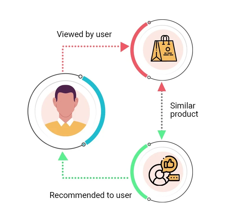
The purpose of Data Science (DS) and Artificial Intelligence (AI) is to add value to a business by utilizing data and applying applicable programming skills. In recent years, Netflix, Amazon, Uber Eats, and other companies have made it possible for people to avail certain commodities with only a few clicks while sitting at home. However, in order to provide users with the most authentic experience possible, these platforms have developed recommendation systems that provide users with a variety of options based on their interests and preferences.

In general, recommendation systems are algorithms that curate data and provide consumers with appropriate material. There are three main types of recommendation engines

  1. Collaborative filtering: Collaborative filtering collects data regarding user behavior, activities, and preferences to predict what a person will like, based on their similarity to other users.
  1.  Content-based filtering: This algorithms analyze the possibility of objects being related to each other using statistics, and then offers possible outcomes to the user based on the highest probabilities.
  1. Hybrid of the two. In a hybrid recommendation engine, natural language processing tags can be generated for each product or item (movie, song), and vector equations are used to calculate the similarity of products.

Building a recommendation system using Python

In this blog, we will walk through the process of scraping a web page for data and using it to develop a recommendation system, using built-in python libraries. Scraping the website to extract useful data will be the first component of the blog. Moving on, text transformation will be performed to alter the extracted data and make it appropriate for our recommendation system to use.

Finally, our content-based recommender system will calculate the cosine similarity of each blog with the rest of the blogs and then suggest three comparable blogs for each blog post.

recommendation system steps
Flow for recommendation system using web scrapping

First step: Web scrapping

The purpose of going through the web scrapping process is to teach how to automate data entry for a recommender system. Knowing how to extract data from the internet will allow you to develop skills to create your own dataset using an entire webpage. Now, let us perform web scraping on the blogs page of online.datasciencedojo.com.

In this blog, we will extract relevant information to make up our dataset. From the first page, we will extract the URL, name, and description of each blog. By extracting the URL, we will have access to redirect our algorithm to each blog page and extract the name and description from the metadata.

The code below uses multiple python libraries and extracts all the URLs from the first page. In this case, it will return ten URLs. For building better concepts regarding web scrapping, I would suggest exploring and playing with these libraries to better understand their functionalities.

Note: The for loop is used to extract URLs from multiple pages.

import requests
import lxml.html
from lxml import objectify
from bs4 import BeautifulSoup
#List for storing urls
urls_final = []
#Extract the metadata of the page
for i in range(1):
url = 'https://online.datasciencedojo.com/blogs/?blogpage='+str(i)
reqs = requests.get(url)
soup = BeautifulSoup(reqs.text, 'lxml')
#Temporary lists for storing temporary data
urls_temp_1 = []
urls_temp_2=[]
temp=[]
#From the metadata, get the relevant information.
for h in soup.find_all('a'):
a = h.get('href')
urls_temp_1.append(a)
for i in urls_temp_1:
if i != None :
if 'blogs' in i:
if 'blogpage' in i:
None
else:
if 'auth' in i:
None
else:
urls_temp_2.append(i)
[temp.append(x) for x in urls_temp_2 if x not in temp]
for i in temp:
if i=='https://online.datasciencedojo.com/blogs/':
None
else:
urls_final.append(i)
print(urls_final)
Output
['https://online.datasciencedojo.com/blogs/regular-expresssion-101/',
'https://online.datasciencedojo.com/blogs/python-libraries-for-data-science/',
'https://online.datasciencedojo.com/blogs/shareable-data-quotes/',
'https://online.datasciencedojo.com/blogs/machine-learning-roadmap/',
'https://online.datasciencedojo.com/blogs/employee-retention-analytics/',
'https://online.datasciencedojo.com/blogs/jupyter-hub-cloud/',
'https://online.datasciencedojo.com/blogs/communication-data-visualization/',
'https://online.datasciencedojo.com/blogs/tracking-metrics-with-prometheus/',
'https://online.datasciencedojo.com/blogs/ai-webmaster-content-creators/',
'https://online.datasciencedojo.com/blogs/grafana-for-azure/']

Once we have the URLs, we move towards processing the metadata of each blog for extracting their name and description.

#Getting the name and description
name=[]
descrip_temp=[]
#Now use each url to get the metadata of each blog post
for j in urls_final:
url = j
response = requests.get(url)
soup = BeautifulSoup(response.text)
#Extract the name and description from each blog
metas = soup.find_all('meta')
name.append([ meta.attrs['content'] for meta in metas if 'property' in meta.attrs and meta.attrs['property'] == 'og:title' ])
descrip_temp.append([ meta.attrs['content'] for meta in metas if 'name' in meta.attrs and meta.attrs['name'] == 'description' ])
print(name[0])
print(descrip_temp[0])
Output:
['RegEx 101 - beginner’s guide to understand regular expressions']
['A regular expression is a sequence of characters that specifies a search pattern in a text. Learn more about Its common uses in this regex 101 guide.']

Second step: Text transformation

Similar to any task involving text, exploratory data analysis (EDA) is a fundamental part of any algorithm. In order to prepare data for our recommender system, data must be cleaned and transformed. For this purpose, we will be using built-in python libraries to remove stop words and transform data.

The code below uses the regex library to perform text transformation by removing punctuations, emojis, and more. Furthermore, we have imported a natural language toolkit (nlkt) to remove stop words.

Note: Stop words are a set of commonly used words in a language. Examples of stop words in English are “a”, “the”, “is”, “are” etc. They are so frequently used in the text that they hold a minimal amount of useful information.

import nltk
from nltk.corpus import stopwords
nltk.download("stopwords")
import re
#Removing stop words and cleaning data
stop_words = set(stopwords.words("english"))
descrip=[]
for i in descrip_temp:
for j in i:
text = re.sub("@\S+", "", j)
text = re.sub(r'[^\w\s]', '', text)
text = re.sub("\$", "", text)
text = re.sub("@\S+", "", text)
text = text.lower()
descrip.append(text)

Following this, we will be creating a bag of words. If you are not familiar with it, a bag of words is a representation of text that describes the occurrence of words within a document. It involves two things: A vocabulary of known words, and a measure of the presence of those words. For our data, it will represent all the keywords words in the dataset and calculate which words are used in each blog and the number of occurrences they have. The code below uses a built-in function to extract keywords.

from keras.preprocessing.text import Tokenizer
#Building BOW
model = Tokenizer()
model.fit_on_texts(descrip)
bow = model.texts_to_matrix(descrip, mode='count')
bow_keys=f'Key : {list(model.word_index.keys())}'

For building better concepts, here are all the extracted keywords.

"Key : ['data', 'analytics', 'science', 'hr', 'azure', 'use', 'analysis', 'dojo',
'launched', 'offering', 'marketplace', 'learn', 'libraries', 'article', 'machine', 'learning', 'work', 'trend', 'insights', 'step',
'help', 'set', 'content', 'creators', 'webmasters', 'regular', 'expression', 'sequence', 'characters', 'specifies', 'search', 'pattern',
'text', 'common', 'uses', 'regex', '101', 'guide', 'blog', 'covers', '6', 'famous', 'python', 'easy', 'extensive', 'documentation',
'perform', 'computations', 'faster', 'enlists', 'quotes', 'analogy', 'importance', 'adoption', 'wrangling', 'privacy', 'security', 'future',
'find', 'start', 'journey', 'kinds', 'projects', 'along', 'way', 'succeed', 'complex', 'field', 'classification', 'regression', 'tree',
'applied', 'companys', 'great', 'resignation', 'era', 'economic', 'triggered', 'covid19', 'pandemic', 'changed', 'relationship', 'offices',
'workers', 'explains', 'overcoming', 'refers', 'collection', 'employee', 'reporting', 'actionable', 'click', 'code', 'explanation', 'jupyter',
'hub', 'preinstalled', 'exploration', 'modeling', 'instead', 'loading', 'clients', 'bullet', 'points', 'longwinded', 'firms',
'visualization', 'tools', 'illustrate', 'message', 'prometheus', 'powerful', 'monitoring', 'alert', 'system', 'artificial', 'intelligence',
'added', 'ease', 'job', 'wonder', 'us', 'introducing', 'different', 'inventions', 'ai', 'helping', 'grafanas', 'harvest', 'leverages', 'power',
'microsoft', 'services', 'visualize', 'query', 'alerts', 'promoting', 'teamwork', 'transparency']"

The code below assigns each keyword an index value and calculates the frequency of each word being used per blog. When building a recommendation system, these keywords and their frequencies for each blog will act as the input. Based on similar keywords, our algorithm will link blog posts together into similar categories. In this case, we will have 10 blogs converted into rows and 139 keywords converted into columns.

import pandas as pd
#Creating df
df_name=pd.DataFrame(name)
df_name.rename(columns = {0:'Blog'}, inplace = True)
df_count=pd.DataFrame(bow)
frames=[df_name,df_count]
result=pd.concat(frames,axis=1)
result=result.set_index('Blog')
result=result.drop([0], axis=1)
for i in range(len(bow)):
result.rename(columns = {i+1:i}, inplace = True)
result
recommendation system input
Input for recommendation system

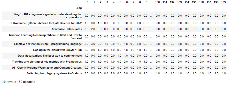
Third step: Cosine similarity

Whenever we are performing some tasks involving natural language processing and want to estimate the similarity between texts, we use some pre-defined metrics that are famous for providing numerical evaluations for this purpose. These metrics include:

  • Euclidean Distance
  • Cosine similarity
  • Jaccard similarity
  • Pearson similarity

While all four of them can be used to evaluate a similarity index between text documents, we will be using cosine similarity for our task. Cosine similarity, in data analysis, measures the similarity between two vectors of an inner product space. It is often used to measure document similarity in text analysis.It measures the cosine of the angle between two vectors and determines a numerical value indicating the probability of those vectors being in the same direction. The code alongside the heatmap shown below visualizes the cosine similarity index for all the blogs.

from sklearn.metrics.pairwise import cosine_similarity
import seaborn as sns
#Calculating cosine similarity
df_name=df_name.convert_dtypes(str)
temp_df=df_name['Blog']
sim_df = pd.DataFrame(cosine_similarity(result, dense_output=True))
for i in range(len(name)):
sim_df.rename(columns = {i:temp_df[i]},index={i:temp_df[i]}, inplace = True)
ax = sns.heatmap(sim_df)
recommendation system heatmap output
Recommendation System Heatmap Output

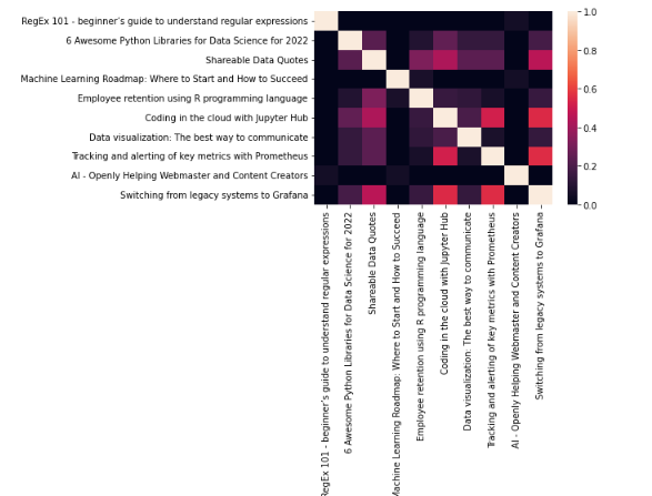
Fourth step: Evaluation

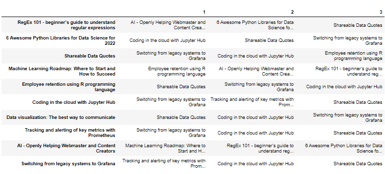
In the code below, our recommender system will extract the three most similar blogs for each blog using Pandas DataFrame.

Note: For each blog, the blog itself is also recommended because it was calculated to be the most similar blog, with the maximum cosine similarity index, 1.

content based recommendation system python ouput
Output for content-based recommendation System Python

Conclusion

This blog post covered a beginner’s method of building a recommendation system using python. While there are other methods to develop recommender systems, the first step is to outline the requirements of the task at hand. To learn more about this, experiment with the code and try to extract data from another web page or enroll in our Python for Data Science course and learn all the required concepts regarding Python fundamentals.

Full Code Available

Data Science Dojo

Recommender systems are one of the most popular algorithms in data science today. Learn how to build a simple movie recommender system.

Recommender systems possess immense capability in various sectors ranging from entertainment to e-commerce. Recommender Systems have proven to be instrumental in pushing up company revenues and customer satisfaction with their implementation. Therefore, machine learning enthusiasts need to get a grasp on it and get familiar with related concepts.

As the amount of available information increases, new problems arise as people are finding it hard to select the items they actually want to see or use. This is where the recommender system comes in. They help us make decisions by learning our preferences or by learning the preferences of similar users.

They are used by almost every major company in some form or the other. Netflix uses it to suggest movies to customers, YouTube uses it to decide which video to play next on autoplay, and Facebook uses it to recommend pages to like and people to follow.

This way recommender systems have helped organizations retain customers by providing tailored suggestions specific to the customer’s needs. According to a study by McKinsey, 35 percent of what consumers purchase on Amazon and 75 percent of what they watch on Netflix come from product recommendations based on such algorithms.

Netflix - Product recommender systems
Audiences watch Netflix and YouTube on recommendations – Recommender systems

Recommender systems can be classified under 2 major categories: Collaborative Systems and Conent-Based Systems.

Collaborative systems

Collaborative systems provide suggestions based on what other similar users liked in the past. By recording the preferences of users, a collaborative system would cluster similar users and provide recommendations based on the activity of users within the same group.

Content-based systems

Content-based systems provide recommendations based on what the user liked in the past. This can be in the form of movie ratings, likes, and clicks. All the recorded activity allows these algorithms to provide suggestions on products if they possess similar features to the products liked by the user in the past.

Content based system
 Content-based systems provide recommendations based on user’s liked content in the past
A hands-on practice, in R, on recommender systems will boost your skills in data science to a great extent. We’ll first practice using the MovieLens 100K Dataset which contains 100,000 movie ratings from around 1000 users on 1700 movies. This exercise will allow you to recommend movies to a particular user based on the movies the user has already rated. We’ll be using the recommender lab package which contains several popular recommendation algorithms.

After completing the first exercise, you’ll have to use the recommenderlab to recommend music to the customers. We use the last.fm dataset that has 92,800 artist listening records from 1892 users. We are going to recommend artists to a user that the user is highly likely to listen.

Install and import required libraries

library(recommenderlab)
library(reshape2)

Import data

The recommenderlab frees us from the hassle of importing the MovieLens 100K dataset. It provides a simple function below that fetches the MovieLens dataset for us in a format that will be compatible with the recommender model. The format of MovieLense is an object of the class “realRatingMatrix” which is a special type of matrix containing ratings. The data will be in the form of a sparse matrix with the movie names in the columns and User IDs in the rows. The interaction of a User ID and a particular movie will provide us with the rating given by that particular user on a scale of 1-5.

As you will see in the output after running the code below, the MovieLense matrix will consist of 943 users (rows) and 1664 movies (columns) with overall 99392 ratings given.

data("MovieLense")
MovieLense
Rating matrix

Data summary

By running the code below, we will visualize a small part of the dataset for our understanding. The code will only display the first 10 rows and 10 columns of our dataset. You can notice that the scores given by the users are integers ranging from 1-5. You’ll also note that most of the values are missing (marked as ‘NA’) indicating that the user hasn’t watched or rated that movie.

ml10 <- MovieLense[c(1:10),]
ml10 <- ml10[,c(1:10)]
as(ml10, "matrix")
MovieLense data matrix
MovieLense data matrix of 100 rows and 100 columns

With the code below, we’ll visualize the MovieLens data matrix of the first 100 rows and 100 columns in the form of a heatmap. Run this code to visualize the movie ratings with respect to a combination of respective rows and columns.

image(MovieLense[1:100,1:100])
heatmap
Visualize movie ratings in the form of a heatmap

Train

We will now train our model using recommenderlab‘s Recommender function is below. The function learns a recommender model from the given data. In this case, our data is the MovieLens data. In the parameters, we are going to specify one of the several algorithms offered by recommenderlab for learning. Here we’ll choose UBCF – User-based Collaborative-Filtering. Collaborative filtering uses given rating data by many users for many items as the basis for predicting missing ratings and/or for creating a top-N recommendation list for a given user, called the active user.

train <- MovieLense
our_model <- Recommender(train, method = "UBCF")
our_model #storing our model in our_model variable

Collaborative filtering

Predict

We will now move ahead and create predictions. From our interaction matrix which is in our dataset MovieLens, we will predict the score for the movies the user hasn’t rated using our recommender model and list the top-scoring movies that our model scored. We will use recommenderlab’s predict function that creates recommendations using a recommender model, our_model in this case, and data about new users.

We will be predicting for a specified user. Below, we have specified a user with ID 115. We have also set n = 10 as our parameter to limit the response to the top 10 ratings given by our model. These will be the movies our model will recommend to the specified user based on his previous ratings.

User = 115
pre <- predict(our_model, MovieLense[User], n = 10)
pre

predicting model to specified user- recommending

List already liked

In the code below we will list the movies the user has already rated and display the score he gave.

user_ratings <- train[User]
as(user_ratings, "list")
List of movies user liked - for recommender system
Movies list rated by users

View result

In the code below, we will display the predictions created in our pre-variable. We will display it in the form of a list.

as(pre,"list")

predictions of pre variable

Conclusion

Using the recommenderlab library we just created a movie recommender system based on the collaborative filtering algorithm. We have successfully recommended 10 movies that the user is likely to prefer. The recommenderlab library could be used to create recommendations using other datasets apart from the MovieLens dataset. The purpose of the exercise above was to provide you with a glimpse of how these models function.

Practice with lastFM dataset

For more practice with recommender systems, we will now recommend artists to our users. We will use the LastFM dataset. This dataset contains social networking, tagging, and music artist listening information from a set of 2K users from Last.fm online music system. It contains almost 92,800 artist listening records from 1892 users.

We will again use the recommenderlab library to create our recommendation model. Since this dataset cannot be fetched using any recommenderlab function as we did for the MovieLens dataset, we will manually fetch the dataset and practice converting it to the realRatingMatrix which is the format that our model will input for modeling.

Below we’ll import 2 files, the user_artists.dat file and artists.dat into the user_artist_data and artist_data variables respectively. The user_artists.dat file is a tab-separated file that contains the artists listened to by each user. It also provides a listening count for each [user, artist] pair marked as attribute weight. The artists.dat file contains information about music artists listened to and tagged by the users. It is a tab-separated file that contains the artist ID, its name, URL, and picture URL.

Let’s import our dataset below:

user_artist_data <- read.csv(file = PATH + "user_artists.dat", header = TRUE, sep="\t")
artist_data <- read.csv(file = PATH + "artists.dat", header = TRUE, sep="\t")

Following the steps we did with our Movie Recommender system, we’ll view the first few rows of our dataset by using the head method.

head(user_artist_data)
Head method
Movie recommender system – head method
We’ll use the head method to view the first 10 rows of the artist dataset below. Think about which columns will be useful for our purpose as we’ll be using a collaborative filtering method for designing our model.
head(artist_data)

head method of 10 rows of artists below

In the code below, we will use the acast method to convert our user_artist dataset into an interaction matrix. This will be later converted to a matrix and then to realRatingMatrix. The realRatingMatrix is the format that will be taken by recommenderlab‘s Recommender function. It is a matrix containing ratings, typically 1-5 stars, etc. We will store in it our rrm_data variable. After running the code, you’ll notice that the output provides us with the dimensions and class of our variable rrm_data.

m_data <- acast(user_artist_data, userID~artistID)
m_data <- as.matrix(m_data)
rrm_data <- as(m_data,"realRatingMatrix")
rrm_data

acast method

Let’s visualize the user_artist data matrix of the first 100 rows and 100 columns in the form of a heatmap. Write a single line code with rrm_data variable to visualize the movie ratings with respect to a combination of respective rows and columns using the image function.

Hint: image(rrm_data[1:100,1:100])
heatmap
Visualize the movie ratings with respect to a combination of respective rows and columns

Using a similar procedure as we used to build our model for the movie recommender system, write a code that builds our Recommender method of the recommenderlab library using the “UBCF” algorithm. Store the model in a variable named artist_model.

We’ll use the predict function to create a prediction for UserID 114 and store the prediction in the variable artist_pre. Also, note that we need the top 12 predictions for listed. The function below will list our prediction using the as method.

train <- rrm_data
artist_model <- Recommender(train, method = "UBCF")
User = 114
artist_pre <- predict(artist_model, rrm_data[User], n = 10)
artist_pre

Recommendations of 1 user

as(artist_pre,"list")

UserID 114

To work with more interesting datasets for recommender systems using recommenderlab or any other relevant library, refer to the article 9 Must-Have Datasets for Investigating Recommender Systems published on kdnuggets.com.


Want to dive deeper into recommender systems? Check out Data Science Dojo’s online data science certificate program.

Related Topics

Statistics
Resources
Programming
Machine Learning
LLM
Generative AI
Data Visualization
Data Security
Data Science
Data Engineering
Data Analytics
Computer Vision
Career
Artificial Intelligence