fbpx
Learn to build large language model applications: vector databases, langchain, fine tuning and prompt engineering. Learn more

scrape data

Data Science Dojo
Syed Umair Hasan
| November 16

A hands-on guide to collect and store twitter data for timeseries analysis 

“A couple of weeks back, I was working on a project in which I had to scrape tweets from twitter and after storing them in a csv file, I had to plot some graphs for timeseries analysis. I requested Twitter for Twitter developer API, but unfortunately my request was not fulfilled. Then I started searching for python libraries which can allow me to scrape tweets without the official Twitter API.

To my amazement, there were several libraries through which you can scrape tweets easily but for my project I found ‘Snscrape’ to be the best library, which met my requirements!” 

What is SNScrape? 

A scraper for social networking platforms known as snscrape (SNS). It retrieves objects, such as pertinent posts, by scraping things like user profiles, hashtags, or searches. 


Install Snscrape 

Snscrape requires Python 3.8 or higher. The Python package dependencies are installed automatically when you install Snscrape. You can install using the following commands. 

  • pip3 install snscrape 

  • pip3 install git+https://github.com/JustAnotherArchivist/snscrape.git (Development Version) 


For this tutorial we will be using the development version of Snscrape. Paste the second command in command prompt(cmd), make sure you have git installed on your system. 


Code walkthrough for scraping

Before starting make sure you have the following python libraries: 

  • Pandas 
  • Numpy 
  • Snscrape 
  • Tqdm 
  • Seaborn 
  • Matplotlit 

Importing Relevant Libraries 

To run the scraping program, you will first need to import the libraries 

import pandas as pd 

import numpy as np 

import snscrape.modules.twitter as sntwitter 

import datetime 

from tqdm.notebook import tqdm_notebook 

import seaborn as sns 

import matplotlib.pyplot as plt 

sns.set_theme(style="whitegrid") 


Taking User Input 

To scrape tweets, you can provide many filters such as the username or start date or end date etc. We will be taking the following user inputs which will then be used in Snscrape. 

  • Text: The query to be matched. (Optional) 
  • Username: Specific username from twitter account. (Required) 
  • Since: Start Date in this format yyyy-mm-dd. (Optional) 
  • Until: End Date in this format yyyy-mm-dd. (Optional) 
  • Count: Max number of tweets to retrieve. (Required) 
  • Retweet: Include or Exclude Retweets. (Required) 
  • Replies: Include or Exclude Replies. (Required) 


For this tutorial we used the following inputs: 

text = input('Enter query text to be matched (or leave it blank by pressing enter)') 

username = input('Enter specific username(s) from a twitter account without @ (or leave it blank by pressing enter): ') 

since = input('Enter startdate in this format yyyy-mm-dd (or leave it blank by pressing enter): ') 

until = input('Enter enddate in this format yyyy-mm-dd (or leave it blank by pressing enter): ') 

count = int(input('Enter max number of tweets or enter -1 to retrieve all possible tweets: ')) 

retweet = input('Exclude Retweets? (y/n): ') 

replies = input('Exclude Replies? (y/n): ') 


Which field can we Scrape? 

Here is the list of fields which we can scrape using Snscrape Library. 

  • url: str 
  • date: datetime.datetime 
  • rawContent: str 
  • renderedContent: str 
  • id: int 
  • user: ‘User’ 
  • replyCount: int 
  • retweetCount: int 
  • likeCount: int 
  • quoteCount: int 
  • conversationId: int 
  • lang: str 
  • source: str 
  • sourceUrl: typing.Optional[str] = None 
  • sourceLabel: typing.Optional[str] = None 
  • links: typing.Optional[typing.List[‘TextLink’]] = None 
  • media: typing.Optional[typing.List[‘Medium’]] = None 
  • retweetedTweet: typing.Optional[‘Tweet’] = None 
  • quotedTweet: typing.Optional[‘Tweet’] = None 
  • inReplyToTweetId: typing.Optional[int] = None 
  • inReplyToUser: typing.Optional[‘User’] = None 
  • mentionedUsers: typing.Optional[typing.List[‘User’]] = None 
  • coordinates: typing.Optional[‘Coordinates’] = None 
  • place: typing.Optional[‘Place’] = None 
  • hashtags: typing.Optional[typing.List[str]] = None 
  • cashtags: typing.Optional[typing.List[str]] = None 
  • card: typing.Optional[‘Card’] = None 


For this tutorial we will not scrape all the fields but a few relevant fields from the above list. 

The search function

Next, we will define a search function which takes in the following inputs as arguments and creates a query string to be passed inside SNS twitter search scraper function. 

  • Text 
  • Username 
  • Since 
  • Until 
  • Retweet 
  • Replies 


def search(text,username,since,until,retweet,replies): 

    global filename 

    q = text 

    if username!='': 

        q += f" from:{username}"     

    if until=='': 

        until = datetime.datetime.strftime(datetime.date.today(), '%Y-%m-%d') 

    q += f" until:{until}" 

    if since=='': 

        since = datetime.datetime.strftime(datetime.datetime.strptime(until, '%Y-%m-%d') -  

                                           datetime.timedelta(days=7), '%Y-%m-%d') 

    q += f" since:{since}" 

    if retweet == 'y': 

        q += f" exclude:retweets" 

    if replies == 'y': 

        q += f" exclude:replies" 

    if username!='' and text!='': 

        filename = f"{since}_{until}_{username}_{text}.csv" 

    elif username!="": 

        filename = f"{since}_{until}_{username}.csv" 

    else: 

        filename = f"{since}_{until}_{text}.csv" 

    print(filename) 

    return q 


Here we have defined different conditions and based on those conditions we are creating the query string. For example, if variable until (end date) is empty then we are assigning it the current date and appending it in a query string and if the variable since (start date) is empty then we are assigning it a date of past 7 days from the current date. Along with the query string, we are creating filename string which will be used to name our csv file. 


Calling the Search Function and creating Dataframe 


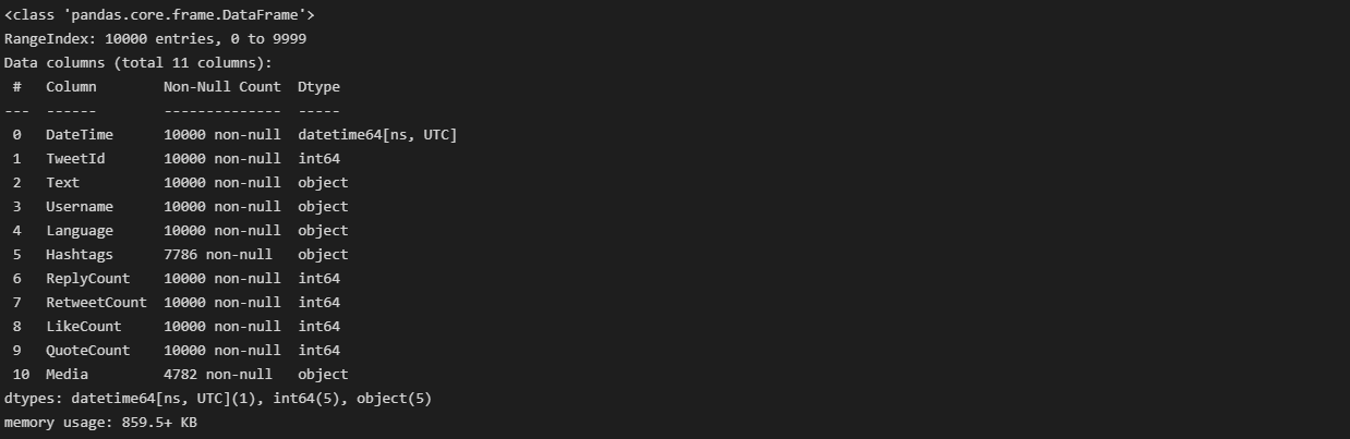
q = search(text,username,since,until,retweet,replies) 

# Creating list to append tweet data  

tweets_list1 = [] 


# Using TwitterSearchScraper to scrape data and append tweets to list 

if count == -1: 

    for i,tweet in enumerate(tqdm_notebook(sntwitter.TwitterSearchScraper(q).get_items())): 

        tweets_list1.append([tweet.date, tweet.id, tweet.rawContent, tweet.user.username,tweet.lang, 

        tweet.hashtags,tweet.replyCount,tweet.retweetCount, tweet.likeCount,tweet.quoteCount,tweet.media]) 

else: 

    with tqdm_notebook(total=count) as pbar: 

        for i,tweet in enumerate(sntwitter.TwitterSearchScraper(q).get_items()): #declare a username  

            if i>=count: #number of tweets you want to scrape 

                break 

            tweets_list1.append([tweet. Date, tweet.id, tweet.rawContent, tweet.user.username,tweet.lang,tweet.hashtags,tweet.replyCount, 

                                tweet.retweetCount,tweet.likeCount,tweet.quoteCount,tweet.media]) 

            pbar.update(1) 

# Creating a dataframe from the tweets list above  

tweets_df1 = pd.DataFrame(tweets_list1, columns=['DateTime', 'TweetId', 'Text', 'Username','Language', 

                                'Hashtags','ReplyCount','RetweetCount','LikeCount','QuoteCount','Media']) 


In this snippet we have invoked the search function and the query string is stored inside variable ‘q’. Next, we have defined an empty list which will be used for appending tweet data. If the count is specified as -1 then the for loop will iterate over all the tweets.

TwitterSearchScraper class constructor takes the query string as an argument and then we invoke the get_items() method of TwitterSearchScraper class to retrieve all the tweets. Inside for loop we append scraped data in the tweets_list1 variable which we defined earlier. If count is defined, then we use it to break the for loop. Finally, using this list, we create the pandas dataframe by specifying the column names. 


tweets_df1.sort_values(by='DateTime',ascending=False) 
Data frame - Panda's library
Data frame created using Panda’s library


Data Preprocessing

Before saving the data frame in a csv file, we will first process the data, so that we can easily perform analysis on it. 


Data Description 

tweets_df1.info() 
Data frame - Panda's library
Data frame created using Panda’s library


Data Transformation 

Now we will add more columns to facilitate timeseries analysis 

tweets_df1['Hour'] = tweets_df1['DateTime'].dt.hour 

tweets_df1['Year'] = tweets_df1['DateTime'].dt.year   

tweets_df1['Month'] = tweets_df1['DateTime'].dt.month 

tweets_df1['MonthName'] = tweets_df1['DateTime'].dt.month_name() 

tweets_df1['MonthDay'] = tweets_df1['DateTime'].dt.day 

tweets_df1['DayName'] = tweets_df1['DateTime'].dt.day_name() 

tweets_df1['Week'] = tweets_df1['DateTime'].dt.isocalendar().week 


The Datetime column contains both date and time, therefore it is better to split data and time in separate columns. 

tweets_df1['Date'] = [d.date() for d in tweets_df1['DateTime']] 

tweets_df1['Time'] = [d.time() for d in tweets_df1['DateTime']] 


After splitting we will drop the DateTime column. 

tweets_df1.drop('DateTime',axis=1,inplace=True) 

tweets_df1 


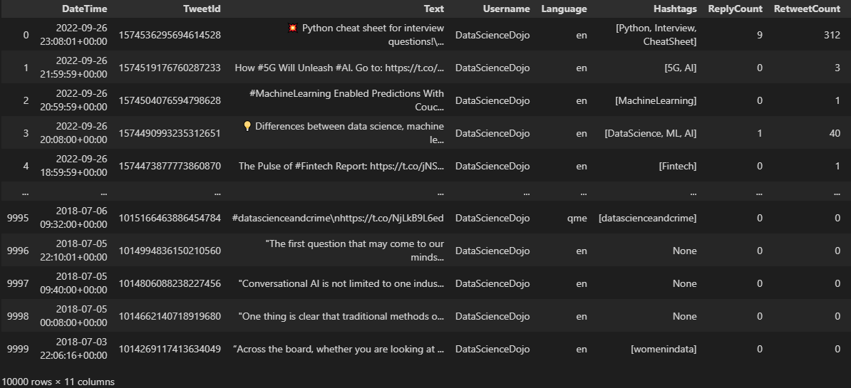
Finally our data is prepared, we will now save the dataframe as csv using df.to_csv() function which takes filename as an input parameter. 

tweets_df1.to_csv(f"{filename}",index=False)

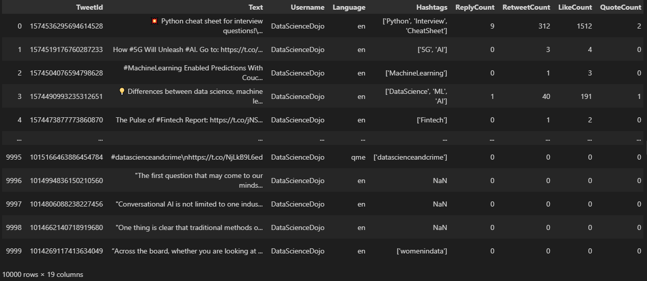
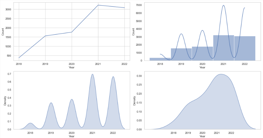
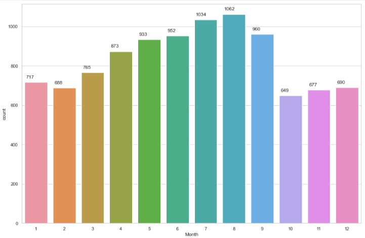
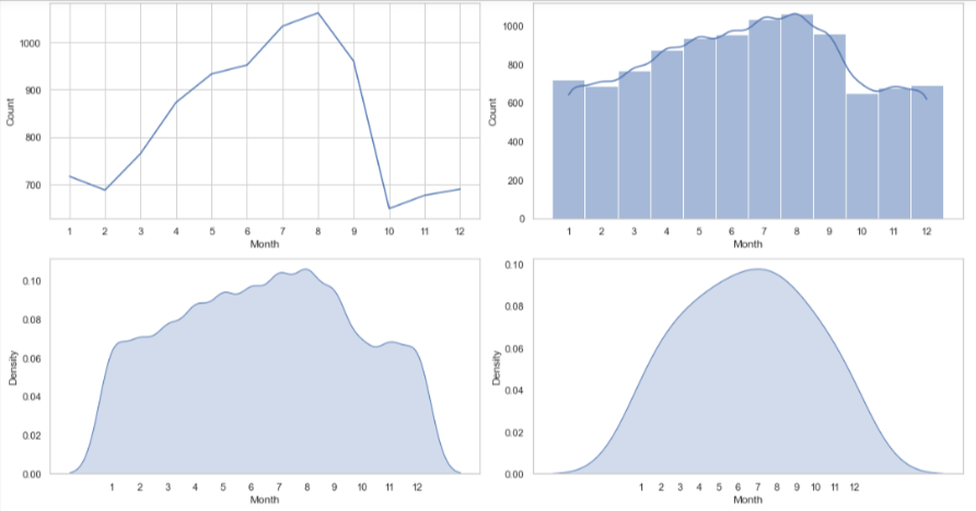
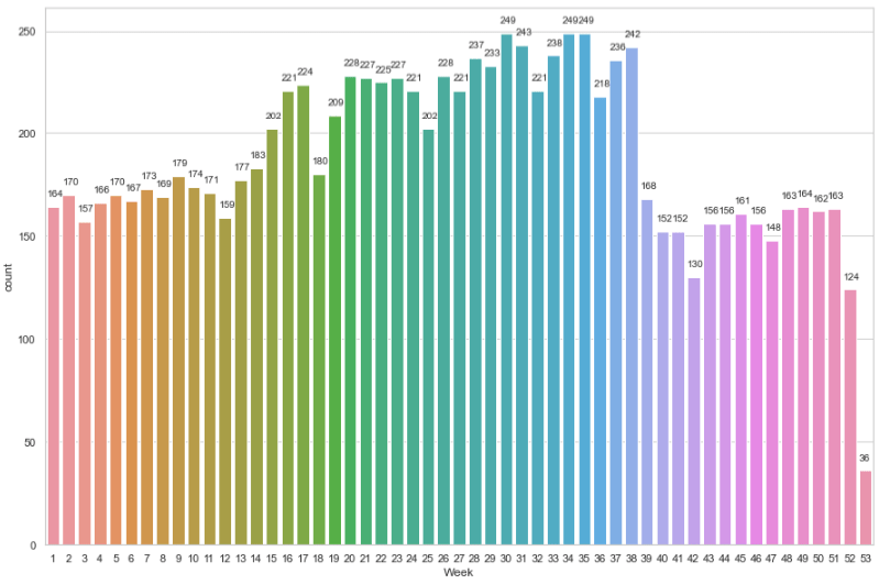
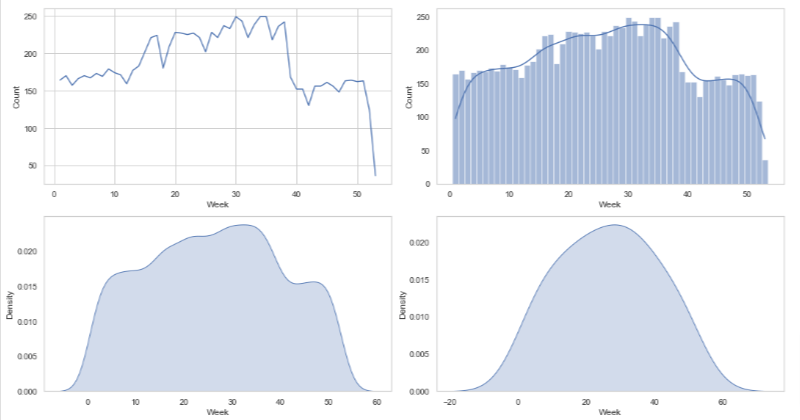
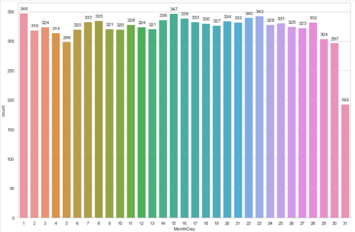
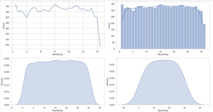
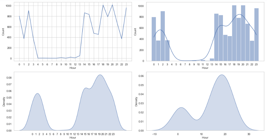
Visualizing timeseries data using barplot, lineplot, histplot and kdeplot 

It is time to visualize our prepared data so that we can find useful insights. Firstly, we will load the saved csv in a dateframe using the read_csv() function of pandas which take filename as input parameter. 

tweets = pd.read_csv("2018-01-01_2022-09-27_DataScienceDojo.csv") 

tweets 


Data frame - Panda's library
Data frame created using Panda’s library


Count by Year 

The countplot function of seaborn allows us to plot count of tweets by year. 

f, ax = plt.subplots(figsize=(15, 10)) 

sns.countplot(x= tweets['Year']) 

for p in ax.patches: 

    ax.annotate(int(p.get_height()), (p.get_x()+0.05, p.get_height()+20), fontsize = 12) 

 
Plot count of tweets - Bar graph
Plot count of tweets – Bar graph


plt.figure(figsize=(15, 8)) 


ax=plt.subplot(221) 

sns.lineplot(tweets.Year.value_counts()) 

ax.set_xlabel("Year") 

ax.set_ylabel('Count') 

plt.xticks(np.arange(2018,2023,1)) 


plt.subplot(222) 

sns.histplot(x=tweets.Year,stat='count',binwidth=1,kde='true',discrete=True) 

plt.xticks(np.arange(2018,2023,1)) 

plt.grid() 


plt.subplot(223) 

sns.kdeplot(x=tweets.Year,fill=True) 

plt.xticks(np.arange(2018,2023,1)) 

plt.grid() 


plt.subplot(224) 

sns.kdeplot(x=tweets.Year,fill=True,bw_adjust=3) 

plt.xticks(np.arange(2018,2023,1)) 

plt.grid() 


plt.tight_layout() 

plt.show() 


Plot count of tweets - per year
Plot count of tweets – per year


Count by Month 

We will follow the same steps for count by month, by week, by day of month and by hour. 


f, ax = plt.subplots(figsize=(15, 10)) 

sns.countplot(x= tweets['Month']) 

for p in ax.patches: 

    ax.annotate(int(p.get_height()), (p.get_x()+0.05, p.get_height()+20), fontsize = 12) 

 
Monthly Tweet counts - chart
Monthly Tweet counts – chart


plt.figure(figsize=(15, 8)) 


ax=plt.subplot(221) 

sns.lineplot(tweets.Month.value_counts()) 

ax.set_xlabel("Month") 

ax.set_ylabel('Count') 

plt.xticks(np.arange(1,13,1)) 


plt.subplot(222) 

sns.histplot(x=tweets.Month,stat='count',binwidth=1,kde='true',discrete=True) 

plt.xticks(np.arange(1,13,1)) 

plt.grid() 


plt.subplot(223) 

sns.kdeplot(x=tweets.Month,fill=True) 

plt.xticks(np.arange(1,13,1)) 

plt.grid() 


plt.subplot(224) 

sns.kdeplot(x=tweets.Month,fill=True,bw_adjust=3) 

plt.xticks(np.arange(1,13,1)) 

plt.grid() 


plt.tight_layout() 

plt.show() 


Monthly tweets count chart


Count by Week 

f, ax = plt.subplots(figsize=(15, 10)) 

sns.countplot(x= tweets['Week']) 

for p in ax.patches: 

    ax.annotate(int(p.get_height()), (p.get_x()+0.005, p.get_height()+5), fontsize = 10) 


Weekly tweets count chart


plt.figure(figsize=(15, 8)) 


ax=plt.subplot(221) 

sns.lineplot(tweets.Week.value_counts()) 

ax.set_xlabel("Week") 

ax.set_ylabel('Count') 


plt.subplot(222) 

sns.histplot(x=tweets.Week,stat='count',binwidth=1,kde='true',discrete=True) 

plt.grid() 


plt.subplot(223) 

sns.kdeplot(x=tweets.Week,fill=True) 

plt.grid() 


plt.subplot(224) 

sns.kdeplot(x=tweets.Week,fill=True,bw_adjust=3) 

plt.grid() 


plt.tight_layout() 

plt.show()  


Weekly tweets count charts


Count by Day of Month 

f, ax = plt.subplots(figsize=(15, 10)) 

sns.countplot(x= tweets['MonthDay']) 

for p in ax.patches: 

    ax.annotate(int(p.get_height()), (p.get_x()+0.05, p.get_height()+5), fontsize = 12) 


Daily tweets count chart
plt.figure(figsize=(15, 8)) 


ax=plt.subplot(221) 

sns.lineplot(tweets.MonthDay.value_counts()) 

ax.set_xlabel("MonthDay") 

ax.set_ylabel('Count') 


plt.subplot(222) 

sns.histplot(x=tweets.MonthDay,stat='count',binwidth=1,kde='true',discrete=True) 

plt.grid() 


plt.subplot(223) 

sns.kdeplot(x=tweets.MonthDay,fill=True) 

plt.grid() 


plt.subplot(224) 

sns.kdeplot(x=tweets.MonthDay,fill=True,bw_adjust=3) 

plt.grid() 


plt.tight_layout() 

plt.show() 


Daily tweets count charts


Count by Hour 

f, ax = plt.subplots(figsize=(15, 10)) 

sns.countplot(x= tweets['Hour']) 

for p in ax.patches: 

    ax.annotate(int(p.get_height()), (p.get_x()+0.05, p.get_height()+20), fontsize = 12) 
hourly tweets count chart


plt.figure(figsize=(15, 8)) 


ax=plt.subplot(221) 

sns.lineplot(tweets.Hour.value_counts()) 

ax.set_xlabel("Hour") 

ax.set_ylabel('Count') 

plt.xticks(np.arange(0,24,1)) 


plt.subplot(222) 

sns.histplot(x=tweets.Hour,stat='count',binwidth=1,kde='true',discrete=True) 

plt.xticks(np.arange(0,24,1)) 

plt.grid() 


plt.subplot(223) 

sns.kdeplot(x=tweets.Hour,fill=True) 

plt.xticks(np.arange(0,24,1)) 

plt.grid() 


plt.subplot(224) 

sns.kdeplot(x=tweets.Hour,fill=True,bw_adjust=3) 

#plt.xticks(np.arange(0,24,1)) 

plt.grid() 


plt.tight_layout() 

plt.show() 


Hourly tweets count charts


Conclusion 

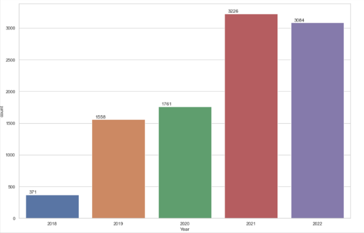
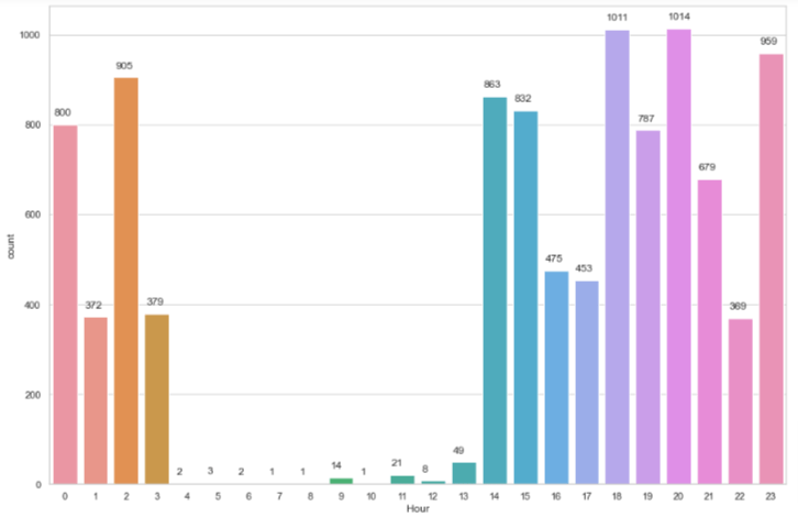
From the above time series visualizations, we can clearly understand that the peak hours of tweets from this account is between 7pm-9pm and from 4am -1pm the twitter handle is quiet. We can also point out that most of the tweets related to that topic are done in the month of August. Similarly, we can identify that the Twitter handle was not very active before 2021.  

Conclusively, we saw how we can easily scrape tweets without using Twitter API through Snscrape. Then we performed some transformations on the scraped data and stored it in csv file. Later, we used that csv file for time-series visualizations and analysis. We appreciate you following along with this hands-on guide. We hope that this guide will make it easy for you to get started on your upcoming data science project. 

<<Link to Complete Code>> 

Related Topics

Statistics
Resources
Programming
Machine Learning
LLM
Generative AI
Data Visualization
Data Security
Data Science
Data Engineering
Data Analytics
Computer Vision
Career
Artificial Intelligence