fbpx
Learn to build large language model applications: vector databases, langchain, fine tuning and prompt engineering. Learn more

Predictive model

Data Science Dojo
Phuc Duong
| March 15

This Azure tutorial will walk you through deploying a predictive model in Azure Machine Learning, using the Titanic dataset.

The classification model, covered in this article, uses the Titanic dataset to predict whether a passenger will live or die, based on demographic information. We’ve already built the model for you and the front-end UI. This tutorial will show you how to customize the Titanic model we built and deploy your own version.
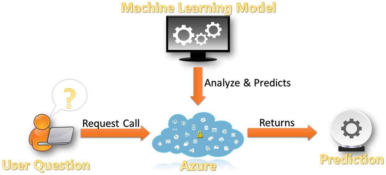
MLaaS overview:

About the data

The Titanic dataset’s complexity scales up with feature engineering, making it one of the few datasets good for both beginners and experts. There are numerous public resources to obtain the Titanic dataset, however, the most complete (and clean) version of the data can be obtained from Kaggle, specifically their “train” data.

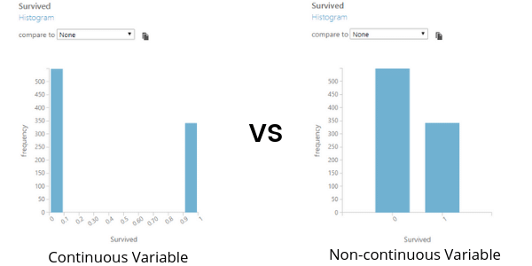
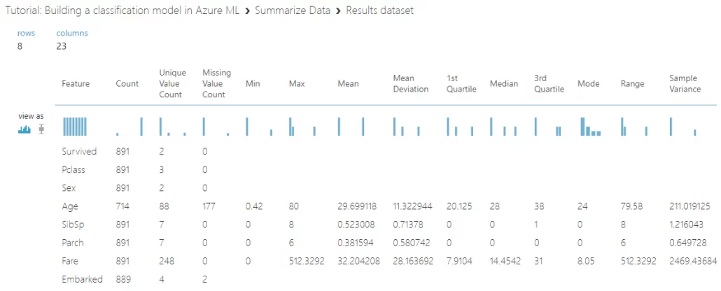
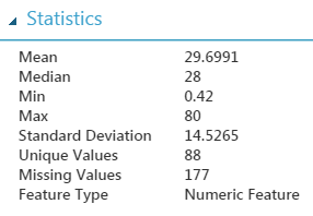
The “train” Titanic data ships with 891 rows, each one about a passenger on the RMS Titanic, the night of the disaster. The dataset also has 12 columns that record attributes of each passenger’s circumstances and demographics such as passenger id, passenger class, age, gender, name, number of siblings and spouses aboard, number of parents and children aboard, fare, ticket number, cabin number, port of embarkation, and whether or not they survived.

For additional reading, a repository of biographies about everyone aboard the RMS Titanic can be found here (complete with pictures).

Titanic route

Getting the experiment

About the titanic survival User Interface

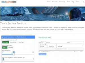
From the dataset, we will build a predictive model and deploy the model in AzureML as a web service. Data Science Dojo has built a front-end UI to interact with such a web service.

Click on the link below to view a finished version of this deployed web service.

Titanic Survival Predictor

Use the app to see what your chance of survival might have been if you were on the Titanic. Play around with the different variables. What factors does the model deem important in calculating your predicted survival rate?

The following tutorial will walk you through how to deploy a titanic prediction model as a web service.


titanic survival predictor

Get an Azure ML account

This MLaaS tutorial assumes that you already have an AzureML workspace. If you do not, please visit the following link for a tutorial on how to create one.

Creating Azure ML Workspace

Please note that an Azure ML 88-hourfree trial does not have the option of deploying a web service.

If you already have an AzureML workspace, then simply visit:

https://studio.azureml.net/

Clone the experiment

For this MLaaS tutorial, we will provide you with the completed experiment by letting you clone ours. If you are curious about how we created the experiment, please view our companion tutorial where we talk about  where we talk about the process of data mining.


clone

Model-Comparison

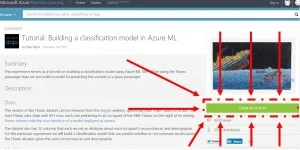
Our experiment is hosted in the Azure ML public gallery. Navigate to the experiment by clicking on the link below or by clicking “Clone ont to Azure ML” within the Titanic Survival Predictor web page itself. The Azure ML Gallery is a place where people can showcase their experiments within the Azure ML community.

Gallery Titanic Experiment

Click on the “open in studio” button.

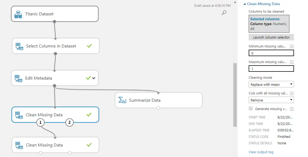
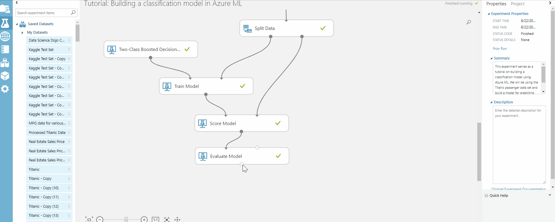
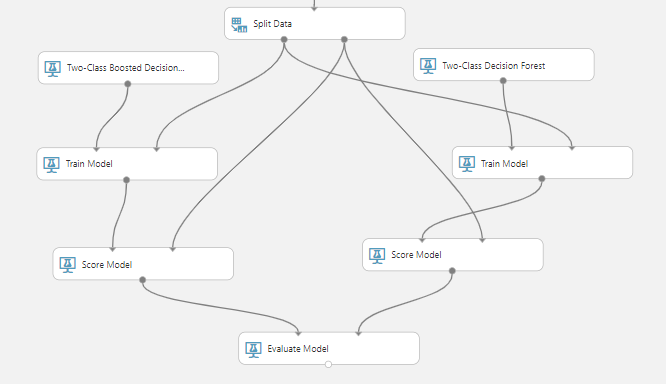
The experiment and dataset will be copied to your studio workspace. You should now see a bunch of modules linked together in a workflow. However, since we have not run the experiment, the workflow only a set of instructions which Azure ML will use to build your models. We will have to run the experiment to produce anything.

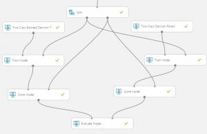
Click the “run” button at the bottom middle of the AzureML window.

This will execute the workflow that is present within the experiment. The experiment will take about 2 minutes and 30 seconds to finish running. Wait until every module has a green checkmark next to it. This indicates that each module has finished running.

MLaaS predictive model evaluation and deployment
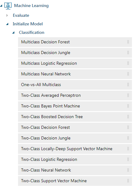
Select an algorithm

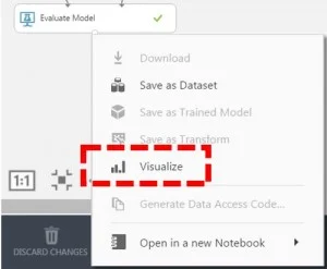
You may have noticed that the cloned experiment shipped with two predictive models–two different decision forests. However, because we can only deploy one predictive model, we should see which performs better. Right click on the output node of the evaluate model module and click “visualize.”


visualize model

Evaluate your model

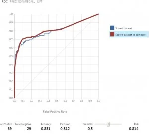
For the purpose of this tutorial, we will define the “better” performing model as the one which scored a higher RoC AuC. We will gloss over evaluating performance metrics of classification models since that would require a longer, more in-depth discussion.

In the evaluate model module, you will see a “ROC” graph with a blue and red line graphed on it. The blue line represents the RoC performance of the model on the left and the red line represents the performance of the model on the right.The higher the curve is on the graph, the better the performance. Since the red curve, the right model, is higher on the graph than the blue curve, we can say that the right model is the better performing model in this case. We will now deploy the corresponding decision tree model.


evaluate model

Deploy the experiment

Before deployment, all modules must have a green check mark next to them.

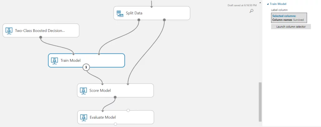
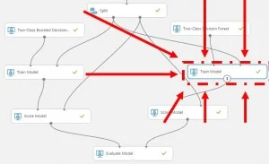
To deploy the selected decision forest model, select the “train model module” on the right.

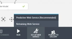
While that is selected, hover over the “setup web service” button on the bottom middle of the screen. A pull-up menu will appear. Select “predictive web service”.

Azure ML will now remove and consolidate unnecessary modules, then it will automatically save the predictive model as a trained model and setup web service inputs and outputs.


train model (1)

deploy model

Drop the response class

Our web service is almost complete. However, we need to tune the logic behind the web service function. The score model module is the module that will execute the algorithm against a given dataset. The score model module can also be called the “prediction module” because that is what happens when you apply a trained algorithm against a dataset.

You will notice that the score model module also takes in a dataset on the right input node. When deploying a predictive model, the score model module will need a copy of the required schema. The dataset used to train the model is fed back into the score model module because that is the schema that our trained algorithm currently knows.

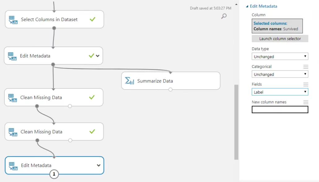
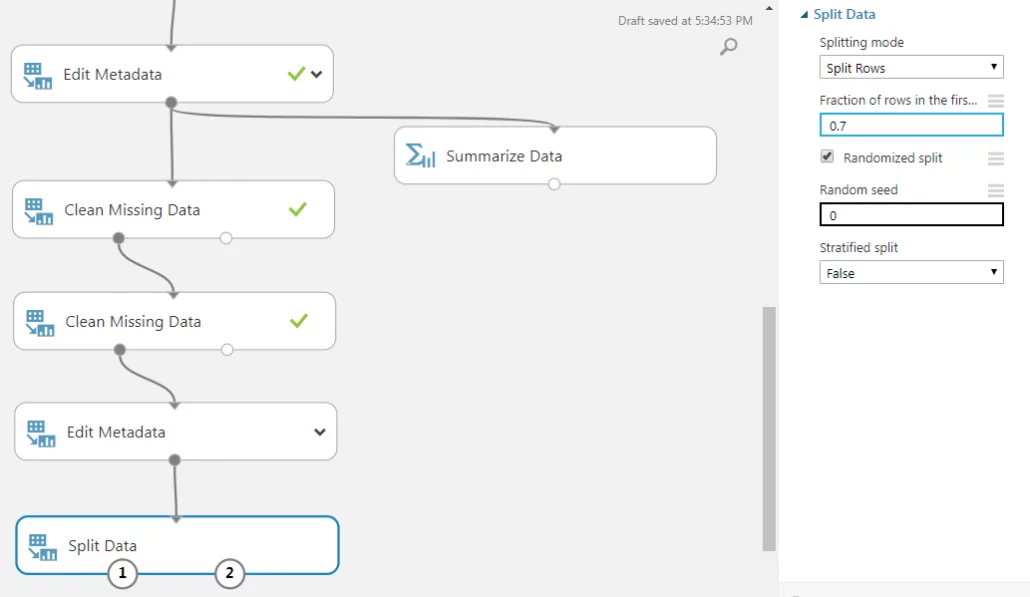
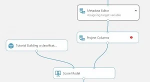
However, that schema also hols our response class “survived,” the attribute that we are trying to predict. We must now drop the survived column. To do this we will use the “project columns” module. Search for it in the search bar on the left side of the AzureML window, then drag it into the workspace.

Replicate the picture on the left by connecting the last metadata editor’s output node to the input of the new project columns module. Then connect the output of the new project columns module with the right input of the score model module.

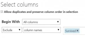
Select the project columns module once the connections have been made. A “properties” window will appear on the right side of the AzureML window. Click on “launch column selector.”

To drop the “Survived” column we will “Begin with: All Columns,” then choose to “Exclude” by “column names,” “Survived.”


drop target

drop target - 1

Reroute web service input

We must now point our web service input in the correct direction. The web service input is currently pointing to the beginning of the workflow where data was cleaned, columns were renamed, and columns were dropped. However, the form on the Titanic Prediction App will do the cleansing for you.

Let’s reroute the web service input to point directly at our score model module. Drag the web service input module down toward the score model module and connect it to the right input node of the score model (the same node that the newly added project columns module is also connected to).

Deploy your model

Once all the rerouting has been done, run your experiment one last time. A “Deploy Web Service” button should now be clickable at the bottom middle of the Azure ML window. Click this and AzureML will automatically create and host your web service API with your own endpoints and post-URL.


deploy model -1

Exposing the deployed webservice


API Diagram


Test your webservice

You should now be on the web deployment screen for your web service. Congratulations! You are now in possession of a web service that is connected to a live predictive model. Let’s test this model to see if it behaves properly.

Click the “test” button in the middle of the web deployment screen. A window with a form should popup. This form should look familiar because it is the same form that the Titanic Predictor App was showing you.

Send the form a few values to see what it returns. The predictions will come in JSON format. The last number in JSON is the prediction itself, which should be a decimal akin to a percentage. This percentage is the predicted likelihood of survival based upon the given parameters, or in this case the passenger’s circumstances while aboard the Titanic.
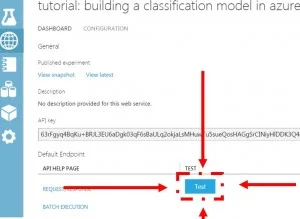
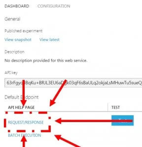
 

test model


Find your API key

The API key is located on the web deployment screen, above the test button that you clicked on earlier. The API key input box comes with a copy to clipboard button, click on that button to copy the key. Paste the key into the “Add Your Own Model” page.
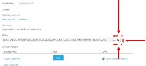
 

find API

Get your post URL

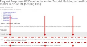
To grab the post-URL, click on the “REQUEST/RESPONSE” button, to the left of the test button. This will take you to the API help page.

Under “Request” and to the right of “POST” is the URL. Copy paste this URL into the “Add Your Own Model” form.


get POST url


get POST url - 1

Enjoy and share

You now have your very own web service! Rememto save the URL because it is your own web page that you may share with others.

If you have a free trial Azure ML account please note that your web service may discontinue when your free trial subscription ends.


Data Science Dojo
Phuc Duong
| August 23

This tutorial will walk you through building a classification model in Azure ML Studio by using the same process as a traditional data mining framework.

Using Azure ML studio (Overview)

We will use the public Titanic dataset for this tutorial. From the dataset, we can build a predictive model that will correctly classify whether you will live or die based upon a passenger’s demographic features and circumstances.

Would you survive the Titanic disaster?

About the data

We use the Titanic dataset in our data science bootcamp, and have found it is one of the few datasets that is good for both beginners and experts because its complexity scales up with feature engineering. There are numerous public resources to obtain the Titanic dataset, however, the most complete (and clean) version of the data can be obtained from Kaggle, specifically their “train” data.

The train Titanic data has 891 rows, each one pertaining to a passenger on the RMS Titanic on the night of its disaster. The dataset also has 12 columns that each record an attribute about each occupant’s circumstances and demographics: user ID, passenger class, age, gender, name, number of siblings and spouses aboard, number of parents and children aboard, fare price, ticket number, cabin number, their port of embarkation, and whether they survived the ordeal or not.

For additional reading, a repository of biographies pertaining to everyone aboard the RMS Titanic can be found here (complete with pictures).

Preprocessing & data exploration

Drop low value columns

Begin by identifying columns that add little-to-no value for predictive modeling. These columns will be dropped.

The first, most obvious candidate to be dropped is PassengerID. No information was provided to us as to how these keys were derived. Therefore, the keys could have been completely random and may add false correlations or noise to our model.

The second candidate for removal is the passenger Name column. Normally, names can be used to derive missing values of gender, but the gender column holds no empty values. Thus, this column is of no use to us, unless we use it to engineer another name column.

The third candidate for removal will be the Ticket column, which represents the ticket serial ID. Much like PassengerID, information is not readily available as to how these ticket strings were derived. Advanced users may dig into historical documents to investigate how the travel agencies set up their ticket names, perform a clustering analysis, or bin the ticket values. Those techniques are out of the scope of this experiment.

The last candidate to be dropped will be Cabin, which is the cabin number where the passenger stayed. Although this column may hold value when binned, there are 147 missing values in this column (~21% of the data). Advanced users may cluster the cabins by letters, or can dig down into the grit of the actual RMS Titanic ship schematics to derive useful features such as cabin distance from hull breach or average elevation from sea level.

Select-Columns
Tutorial: Building a Classification Model in Azure ML

Define categorical variables

We must now define which values are non-continuous by casting them as categorical. Mathematical approaches for continuous and non-continuous values differ greatly. For example, if we graph the “Survived” column now, it will look funny because it would try to account for the range in between “0” and “1”. However, being partially alive in this case would be absurd. Categorical values are looked at independent of one another as “choices” or “options” rather than as a numeric range.

For a quick (but not exhaustive) exercise to see if something should be categorical, simply ask, “Would a decimal interval for this value make sense?”

Continuous-vs-non-continuous
Difference between Continuous and Non-Continuous Variable

From this exercise, the columns that should be cast as categorical are: Survived, Pclass, Sex, and Embarked. The trickiest of these to determine might have been Pclass because it’s a numerical value that goes from 1 to 3. However, it does not really make sense to have a 2.5 Class between second class and third class. Also, the relationship or “distance” between each interval of PClass is not explicit.

To cast these columns, drag in the “Edit Metadata” module. Specify the columns to be cast, then change the “Categorical” parameter to “Make categorical”.

Make-Categorical
Building a Classification Model in Azure ML

Clean missing data in Azure ML

Most algorithms are unable to account for missing values and some treat it inconsistently from others. To address this, we must make sure our dataset contains no missing, “null,” or “NA” values. There are many ways to address missing values. We will cover three: replacement, exclusion, and deletion.

We used exclusion already when we made a conscious decision not to use “Cabin” attributes by dropping the column entirely.

Replacement is the most versatile and preferred method because it allows us to keep our data. It also minimizes collateral damage to other columns as a result of one cell’s bad behavior. In replacement, numerical values can easily be replaced with statistical values such as mean, median, or mode. The median is usually preferred for machine learning because it preserves the distribution of the data and is less affected by outliers. However, the median will skew and overload your frequencies, meaning it’ll mess with your bar graph but not your box plot.

We will cover deletion later in this section.

Now we can hunt for missing values. Drag in a “Summarize Data” module and connect it to your “Edit Metadata” module. Run the experiment and visualize the summary output. You will get a column summarizing “missing value count” for each attribute. At this point, there are 177 missing values for “Age” and 2 missing values for “Embarked.”

Summarize-Data
Dataset Results
clean-missing-data
Cleaning Missing Data

Looking at the metadata of “Age” reveals that it is a “numeric” type. As such, we can easily replace all missing values of age with the median. In this case, each missing value will be replaced with “28.”

Embarked is a bit trickier since it is a categorical string. Usually, the holes in categorical columns can be filled with a placeholder value. In this case, there are only 2 missing values so it would not make much sense to add another categorical value to “Embarked” in the form of S, C, Q, or U (for unknown) just to accommodate 2 rows. We can stand to lose 0.2% of our data by simply dropping these rows. This is an example of deletion.

azure-ml-tutorial--metadata-on-age
Building a Predictive Model using Azure ML – Statistics

To clean missing values in Azure ML, use the “Clean Missing Data” module. This module will apply a single blanket operation to the selected features.  First, we start by having one “Clean Missing Data” module to replace all missing numeric instances with the median.  To select all the numeric columns, we select “Column Type” and “Numeric” under “Launch Column Selector” in the Properties of “Clean Missing Data.”  This will target only the “Age” column since it is the only numeric column with missing values. After the data goes through the module, there should only be 2 missing values left in the entire dataset, which is in “Embarked” column.  Then, we add another “Clean Missing Data” module, set it to drop the missing rows in order to remove the 2 missing values of “Embarked.”

Clean-missing-values
Azure ML – Cleaning Missing Data

Specify a response class

We must now directly tell Azure ML which attribute we want our algorithm to train to predict by casting that attribute as a “label.” Do this by dragging in a “Edit Metadata” module. Use the column selector to specify “Survived” and change the “Fields” parameter to “Labels.” A dataset can only have 1 label at a time for this to work. Our model is now ready for machine learning!

response-class
Azure ML – Specifying a Response Class

Partition and withhold data

It is extremely important to randomly partition your data prior to training an algorithm to test the validity and performance of your model. A predictive model is worthless to us if it can only accurately predict known values. Withhold data represents data that the model never saw when it was training its algorithm. This will allow you to score the performance of your model later to evaluate how well the model can predict future or unknown values.

Drag in a “Split Data” module. It is usually industry practice to set a 70/30 split. To do this, set “fraction of rows in the first output dataset” to be 0.7. 70% of the data will be randomly shuffled into the left output node, while the remaining 30% will be shuffled into the right output node.

spit-data-azure-machinelearning
Azure ML – Splitting Data

Select an algorithm

First, we must identify what kind of machine learning problem this is: classification, regression, clustering, etc. Since the response class is a categorical value, or “0” or “1”, for survived or deceased, we can tell that it is a classification problem. Specifically, we can tell that it is a two-class, or binary, classification problem because there are only two possible results: survived or deceased. Luckily, Azure ML ships with many two-class classification algorithms. Without going into algorithm-specific implementations, this problem lends itself well to decision forest and decision tree because the predictor classes are both numeric and categorical. Pick one algorithm (any two-class algorithm will work).

decision-tree-azure-ml
Selecting an Algorithm in Azure ML

Train your model

Drag in a “Train Model” module and connect your algorithm to it. Connect your training data (the 70%) to the right input of the “Train Model” module. To score the model, drag in a “Score Model” module. Connect the “Train Model” to the left input node of the “Score Model,” and the 30% withhold data to the right input node of the “Score Model.” Finally, to evaluate the performance of model, drag in an “Evaluate Model” module and connect its left input to the output of the “Score Model.”

Run your model

azure-ml-tutorial--training-your-model
Running your Model in Azure ML

Evaluate your model

If you visualize your “Evaluate Model” module after running your model, you see a staggering number of metrics. Each machine learning problem will have its own unique goals, thus having different priorities when evaluating “good” or “bad” performance. As a result, each problem will also optimize different metrics.

For our experiment, we chose to maximize the RoC AuC because this is a low-risk situation where the outcomes of false negatives or false positives do not have different weights.

RoC AuCs will vary slightly because of the randomized split. The default parameters of our two-class boosted decision tree yielded a RoC AuC of 0.832. This is a fair performing model. By fine-tuning the parameters, we can further increase the performance of the model.

Evaluationofmodel
Evaluating your Model in Azure ML

Which metric to optimize?

  1. RoC AuC: Overall Performance
  2. Precision: Relevance
  3. Recall: Thoroughness
  4. Accuracy: Correctness

Beginner’s guide to RoC AuC

  • o.9~1 = Suspiciously Good
  • 0.8~0.9 = Fair
  • 0.7~0.8 = Decent Model
  • 0.5~0.6 = Worthless Model

Compare your model

How would our model shape up against another algorithm? Let’s find out. Drag in a “Two-Class Decision Forest” module. Copy and paste your “Train Model” module and your “Score Model” module. Reroute the input of the newly-created “Train Model” module to the decision forest. Attach the output of the newly-created “Score Model” module to the right input node of the “Evaluate Model” module. Now we can compare the performance of two machine learning models that were trained separately.

compare your model
Comparing your Model in Azure ML

Both models performed fairly (~0.81 RoC AuC each). The boosted decision tree got a slightly higher RoC AuC overall, but the two models were close enough to be considered tied in terms of performance. As a tiebreaker, we can look at other metrics such as accuracy, precision, and recall. Using those metrics, we found that the boosted decision tree had lower accuracy, precision, and recall when compared to the two-class decision forest. If we were to select a winning model right now, it would probably be the two-class decision forest.

Other video tutorials

You can watch this series of videos to dive deeper into Azure Machine Learning:

Related Topics

Statistics
Resources
Programming
Machine Learning
LLM
Generative AI
Data Visualization
Data Security
Data Science
Data Engineering
Data Analytics
Computer Vision
Career
Artificial Intelligence