algorithm

Learn how companies like Zillow predict the value of your home. Build a predictive model using Azure machine learning that estimates the real estate sales price of a house.

Ames housing dataset includes 81 features and 1460 observations. Each observation represents the sale of a home and each feature is an attribute describing the house or the circumstance of the sale.

Clone this experiment to build a predictive model

A full copy of this experiment has been posted to the Cortana Intelligence Gallery. Go to the link and click on “open in Studio.”

Preprocessing & data exploration

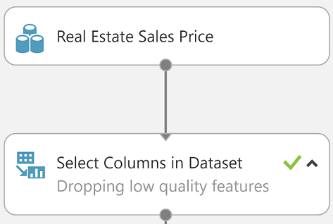
Drop low-value columns

Begin by identifying features (columns) that add little to no value for predictive modeling. These columns will be dropped using the “select columns from dataset” module.

The following columns were chosen to be “excluded” from the dataset:

Id, Street, Alley, PoolQC, Utilities, Condition2, RoofMatl, MiscVal, PoolArea, 3SsnPorch, LowQualFinSF, MiscFeature, LandSlope, Functional, BsmtHalfBath, ScreenPorch, BsmtFinSF2, EnclosedPorch.

These low-quality features were removed to improve the model’s performance. Low quality includes lack of representative categories, too many missing values, or noisy features.

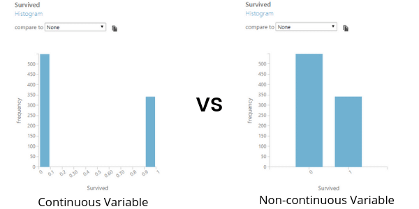
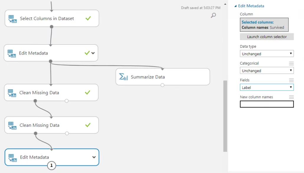
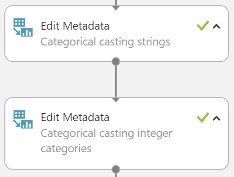
Define categorical variables

We must now define which values are non-continuous by casting them as categorical. Mathematical approaches for continuous and non-continuous values differ greatly. Nominal categorical features were identified and cast to categorical data types using the metadata editor to ensure proper mathematical treatment by the machine learning algorithm.

The first edit metadata module will cast all strings. The column “MSSubClass” uses numeric integer codes to represent the type of building the house is, and therefore should not be treated as a continuous numeric value but rather a categorical feature. We will use another metadata editor to cast it into a category.

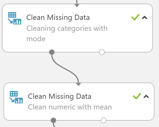
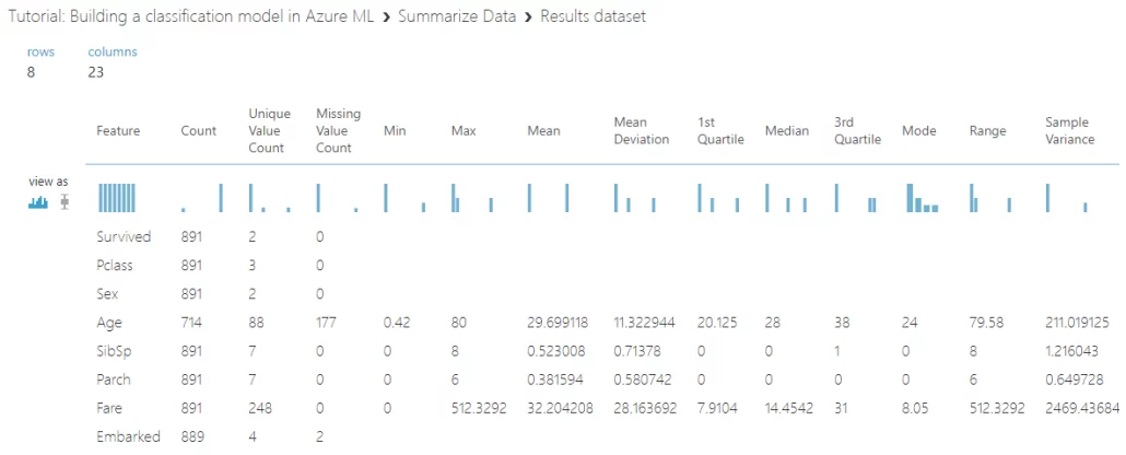
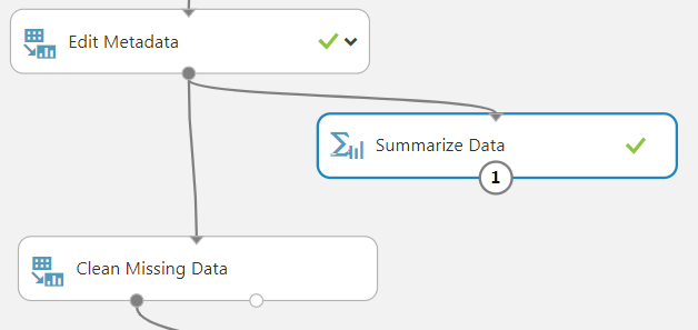
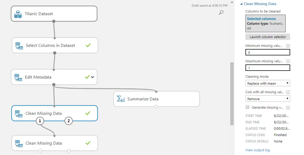
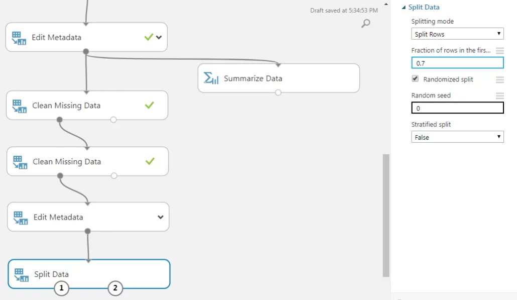
Clean missing data

Most algorithms are unable to account for missing values and some treat it inconsistently from others. To address this, we must make sure our dataset contains no missing, “null,” or “NA” values.

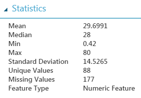
Replacement of missing values is the most versatile and preferred method because it allows us to keep our data. It also minimizes collateral damage to other columns due to one cell’s bad behavior. Numerical values can easily be replaced with statistical values such as mean, median, or mode.

While categories can be commonly dealt with by replacing with the mode or a separate categorical value for unknowns.

For simplicity, all categorical missing values were cleaned with the mode and all numeric features were cleaned using the median. To further improve a model’s performance, custom cleaning functions should be tried and implemented on each individual feature rather than a blanket transformation of all columns.

Machine learning – Model building

Statistical feature selection

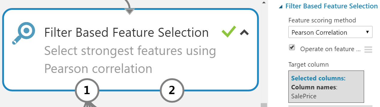
Not every feature in its current form is expected to contain predictive value to the model and may mislead or add noise to the model. To filter these out we will perform a Pearson correlation to test all features against the response class (sales price) as a quick measure of their predictive strength, only picking the top X strongest features from this method, the remaining features will be left behind.

This number can be tuned for further model performance increases.

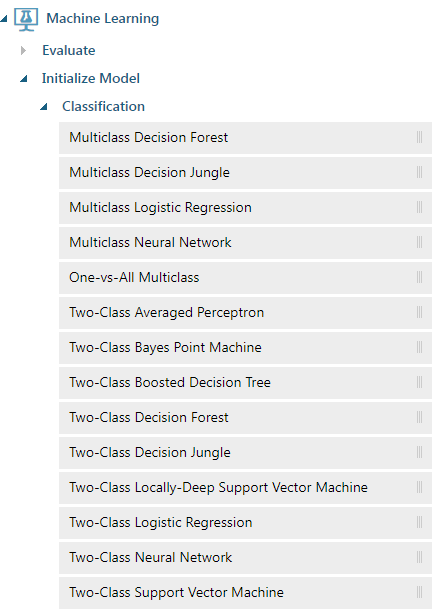
Select an algorithm

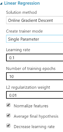
First, we must identify what kind of machine learning problem this is: classification, regression, clustering, etc. Since the response class (sales price) is a continuous numeric value, we can tell that it is a regression problem. We will use a linear regression model with regularization to reduce the over-fitting of the model.

• To ensure a stable convergence of weight and biases, all features except the response class must be normalized to be placed into the same range.

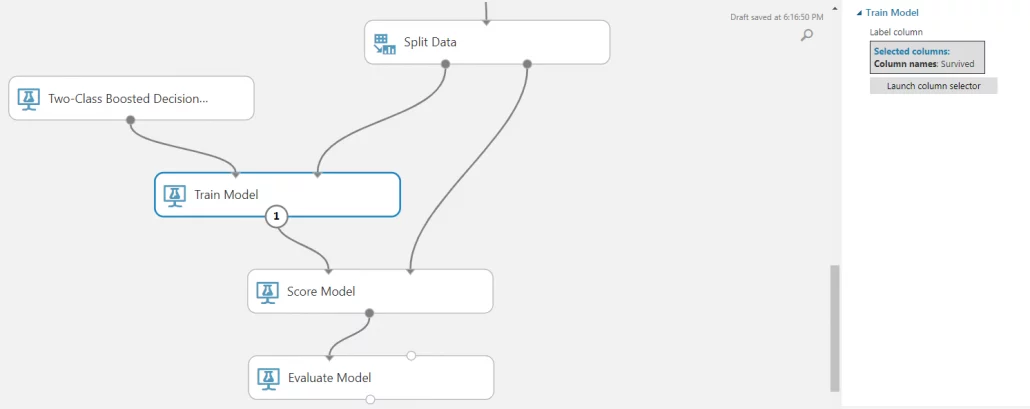
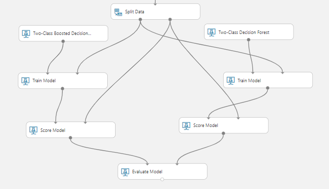
Model training and evaluation

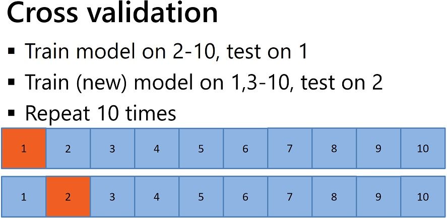
The method of cross-validation will be used to evaluate the predictive performance of the model as well as that performance’s stability in regard to new data. Cross-validation will build ten different models on the same algorithm but with different and non-repeating subsets of the same dataset. The evaluation metrics on each of the ten models will be averaged and a standard deviation will infer the stability of the average performance.

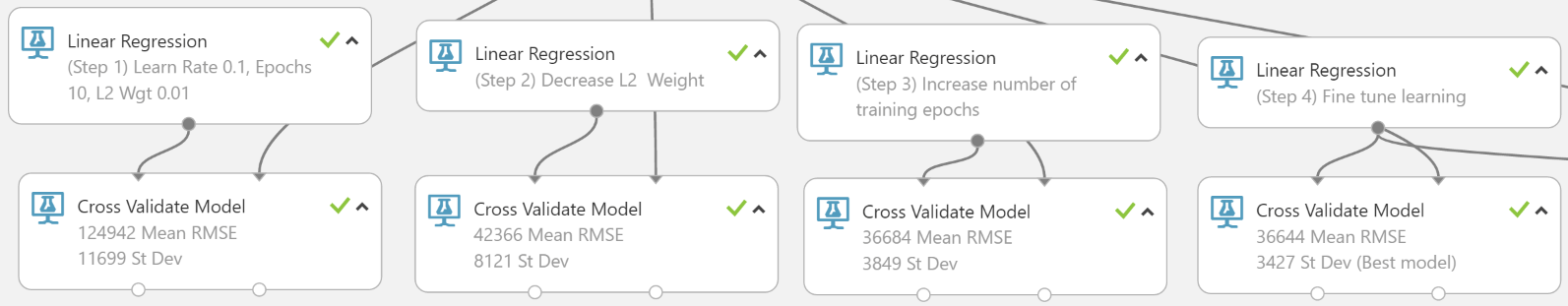
Parameter tuning

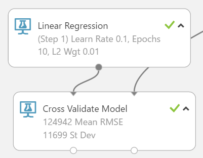
This experiment will build a regression model that minimizes the mean RMSE of the cross-validation results with the lowest variance possible(but also considers bias-variance trade-offs).

1. The first regression model was built using default parameters and produced a very inaccurate model ($124,942 mean RMSE) and was very unstable (11,699 standard deviation).
2. The high bias and high variance of the previous model suggest the model is over-fitting to the outliers and is under-fitting the general population.
3. The L2 regularization weight will be decreased to lower the penalty of higher coefficients. After lowering the L2 regularization weight, the model is more accurate with an average cross-validation RMSE of $42,366.
4. The previous model is still quite unstable with a standard deviation of $8,121. Since this is a dataset with a small number of observations (1460), it may be better to increase the number of training epochs so that the algorithm has more passes to reach convergence.
5. This will increase training times but also increase stability. The third linear model had the number of training epochs increased and saw a better mean cross-validation RMSE of $36,684 and a much more stable standard deviation of $3,849.
6. The final model had a slight increase in the learning rate which improved both mean cross-validation RMSE and the standard deviation.

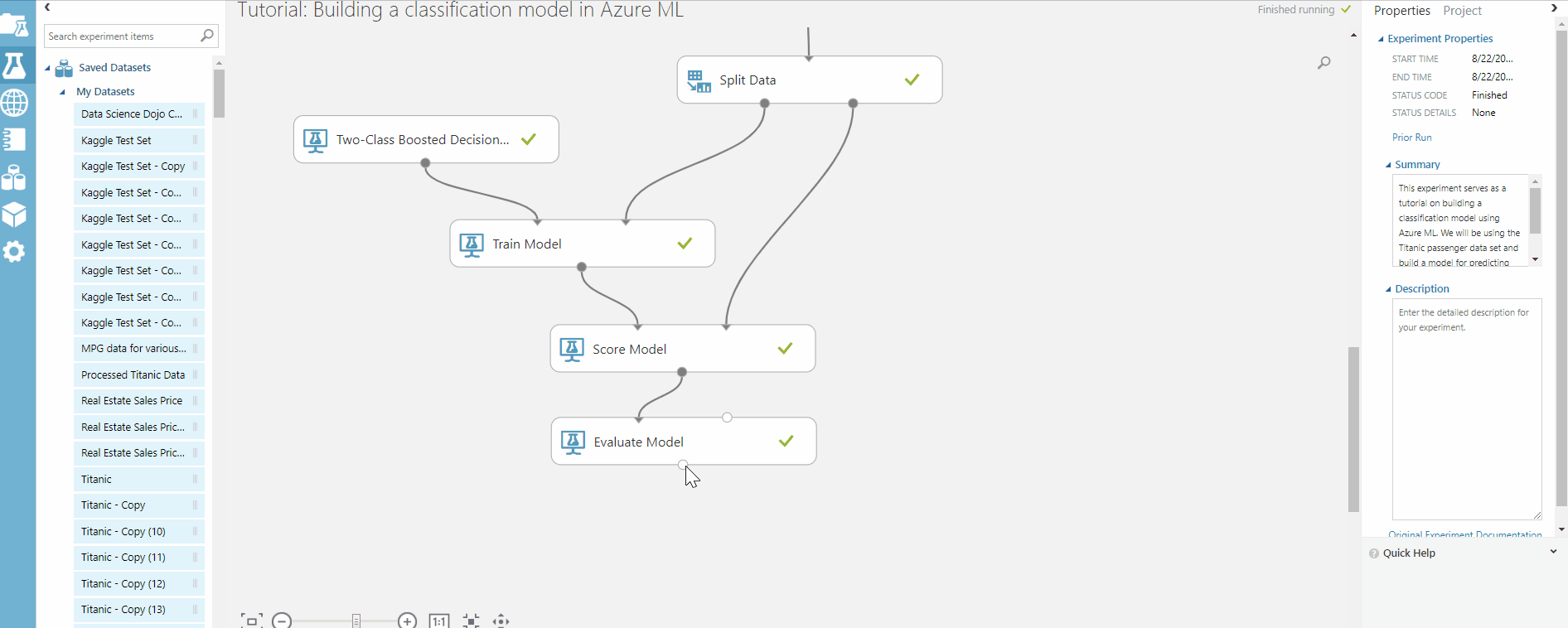
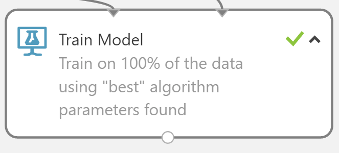
Deployment

The algorithm parameters that yielded the best results will be the ones that are shipped. The best algorithm (the last one) will be retrained using 100% of the data since cross-validation leaves 10% out each time for validation.

Further improvement of this Azure machine learning model

Feature engineering was entirely left out of this experiment. Try engineering more features from the existing dataset to see if the model will improve. Some columns that were originally dropped may become useful when combined with other features. For example, try bucketing the years in which the house was built by decade. Clustering the data may also yield some hidden insights.

Just like humans, algorithms can develop bias and make skewed decisions. What are these biases and how do they impact decision-making?

An algorithmic bias in making

If we took a hard look at every model ever built for classifying who is the optimal candidate for:

• A credit loans
• A job promotion
• A free scholarship or
• Any other opportunity,

would we see a pattern in certain groups of people being granted these opportunities over others? Are our algorithms and formulas biased?

Understanding the problem

Would we see these models repeatedly make decisions about who should be part of the “have” and “have not” groups? Further, do these models truly pick the optimal candidate? Instead, might they pick according to what someone personally thinks is the optimal candidate?

Please note, that it has been argued that algorithms are not completely subjective-free. In fact, just like the humans who develop them, algorithms can come with inherent bias. Some examples of this include rejecting credit loan applications from African Americans and Latin Americans.

Another example includes advertising high-paying jobs to men more often than women. As a result, these incidents have led us to question how companies and governments construct models that influence decisions.

Research groups like AI Now recently launched an initiative to fight algorithmic bias. As a result, it’s bringing the issues to light. It’s crucial that we as data scientists keep our algorithms in check. This is to avoid developing yet another tool that is used to discriminate against people.

So how can we keep our algorithms in check?

In recent years, researchers have come up with ways to detect if a model is biased in its decisions about people. A 2016 paper called Equality of Opportunity in Supervised Learning proposes a framework.

This framework uses “equalized odds and equal opportunity” as a criterion for assessing a model’s fairness when classifying people. This criterion allows features to predict an outcome or class (such as predicting a “high credit risk applicant”).

It prohibits abusing a particular attribute of a person (such as race) to do this. The model must be equally accurate in all demographics. Consequently, it is punished if it only performs well for the majority of people. This means that the predicted outcome must have equal true positive/negative rates and false positive/negative rates across all demographics.

The framework is conducted as a post-learning step. Therefore, it doesn’t require modifying the algorithm or model itself. Then it assesses whether the results from a model seem skewed towards a group of people. For example, a flawed model makes it harder for African Americans who do pay back their loans to apply for loans.

This model makes it easier for Caucasians who don’t pay back their loans to apply for loans. Therefore, this framework ensures that this kind of model would be determined as unfair, as it would not result in equal false positive/negative rates for both African Americans and Caucasians.

The framework also overcomes the problem of loss of utility when using demographic parity. This requires a predicted outcome to be independent of a particular sensitive attribute.

Using the framework, the predicted outcome is allowed to depend on a particular attribute, but only through the actual outcome. This prevents the attribute from being a proxy to the actual outcome while avoiding loss of utility.

Predictor variables and skewed data

Another framework for detecting algorithmic bias is testing how different predictor variables or attributes might skew the predicted outcome. A 2017 paper called Counterfactual Fairness shows how different variables influenced the results of the 2014 stop-and-frisk New York City police initiative.

The data showed that the police officers mostly stopped and frisked African Americans and Hispanics. This happened despite most of those people being innocent or not as suspicious as predicted.

Subsequently, actual incidents of crime were similar across all races. When considering all predictor variables, including the race attribute, the model learned to correlate race with the criminality outcome. Then, the researchers were able to get a more accurate spotting of criminals. Researchers used variables that only related to a person’s criminality.

This was instead of if they had of built a model highly dependent on race and appearance.

The Takeaway

First, this research shows that relying on race as a predictor leads to a skewed outcome. Second, it also shows how ineffective the police would be by allowing such bias to be at the core of their decisions.

Visualizations of the predicted versus the actual data show how some locations with a high number of arrests could be completely missed if they were to depend on race. How we construct our models and the variables we use can truly affect people’s opportunities, livelihood, and overall well-being. Therefore, this must be handled ethically and responsibly.

As data scientists, our philosophy should be built on the pursuit of truth, not the manipulation of models to find the most convenient or profitable results at all costs, even at the cost of our ethics.

We must include bias assessments as part of the process, so we can be more confident that our models are designed to better our understanding of people and make smarter decisions, not dumb and discriminatory decisions.

This tutorial will walk you through building a classification model in Azure ML Studio by using the same process as a traditional data mining framework.

Using Azure ML studio (Overview)

We will use the public Titanic dataset for this tutorial. From the dataset, we can build a predictive model that will correctly classify whether you will live or die based upon a passenger’s demographic features and circumstances.

Would you survive the Titanic disaster?

About the data

We use the Titanic dataset in our data science bootcamp, and have found it is one of the few datasets that is good for both beginners and experts because its complexity scales up with feature engineering. There are numerous public resources to obtain the Titanic dataset, however, the most complete (and clean) version of the data can be obtained from Kaggle, specifically their “train” data.

The train Titanic data has 891 rows, each one pertaining to a passenger on the RMS Titanic on the night of its disaster. The dataset also has 12 columns that each record an attribute about each occupant’s circumstances and demographics: user ID, passenger class, age, gender, name, number of siblings and spouses aboard, number of parents and children aboard, fare price, ticket number, cabin number, their port of embarkation, and whether they survived the ordeal or not.

For additional reading, a repository of biographies pertaining to everyone aboard the RMS Titanic can be found here (complete with pictures).

Preprocessing & data exploration

Drop low value columns

Begin by identifying columns that add little-to-no value for predictive modeling. These columns will be dropped.

The first, most obvious candidate to be dropped is PassengerID. No information was provided to us as to how these keys were derived. Therefore, the keys could have been completely random and may add false correlations or noise to our model.

The second candidate for removal is the passenger Name column. Normally, names can be used to derive missing values of gender, but the gender column holds no empty values. Thus, this column is of no use to us, unless we use it to engineer another name column.

The third candidate for removal will be the Ticket column, which represents the ticket serial ID. Much like PassengerID, information is not readily available as to how these ticket strings were derived. Advanced users may dig into historical documents to investigate how the travel agencies set up their ticket names, perform a clustering analysis, or bin the ticket values. Those techniques are out of the scope of this experiment.

The last candidate to be dropped will be Cabin, which is the cabin number where the passenger stayed. Although this column may hold value when binned, there are 147 missing values in this column (~21% of the data). Advanced users may cluster the cabins by letters, or can dig down into the grit of the actual RMS Titanic ship schematics to derive useful features such as cabin distance from hull breach or average elevation from sea level.

Define categorical variables

We must now define which values are non-continuous by casting them as categorical. Mathematical approaches for continuous and non-continuous values differ greatly. For example, if we graph the “Survived” column now, it will look funny because it would try to account for the range in between “0” and “1”. However, being partially alive in this case would be absurd. Categorical values are looked at independent of one another as “choices” or “options” rather than as a numeric range.

For a quick (but not exhaustive) exercise to see if something should be categorical, simply ask, “Would a decimal interval for this value make sense?”

From this exercise, the columns that should be cast as categorical are: Survived, Pclass, Sex, and Embarked. The trickiest of these to determine might have been Pclass because it’s a numerical value that goes from 1 to 3. However, it does not really make sense to have a 2.5 Class between second class and third class. Also, the relationship or “distance” between each interval of PClass is not explicit.

To cast these columns, drag in the “Edit Metadata” module. Specify the columns to be cast, then change the “Categorical” parameter to “Make categorical”.

Clean missing data in Azure ML

Most algorithms are unable to account for missing values and some treat it inconsistently from others. To address this, we must make sure our dataset contains no missing, “null,” or “NA” values. There are many ways to address missing values. We will cover three: replacement, exclusion, and deletion.

We used exclusion already when we made a conscious decision not to use “Cabin” attributes by dropping the column entirely.

Replacement is the most versatile and preferred method because it allows us to keep our data. It also minimizes collateral damage to other columns as a result of one cell’s bad behavior. In replacement, numerical values can easily be replaced with statistical values such as mean, median, or mode. The median is usually preferred for machine learning because it preserves the distribution of the data and is less affected by outliers. However, the median will skew and overload your frequencies, meaning it’ll mess with your bar graph but not your box plot.

We will cover deletion later in this section.

Now we can hunt for missing values. Drag in a “Summarize Data” module and connect it to your “Edit Metadata” module. Run the experiment and visualize the summary output. You will get a column summarizing “missing value count” for each attribute. At this point, there are 177 missing values for “Age” and 2 missing values for “Embarked.”

Looking at the metadata of “Age” reveals that it is a “numeric” type. As such, we can easily replace all missing values of age with the median. In this case, each missing value will be replaced with “28.”

Embarked is a bit trickier since it is a categorical string. Usually, the holes in categorical columns can be filled with a placeholder value. In this case, there are only 2 missing values so it would not make much sense to add another categorical value to “Embarked” in the form of S, C, Q, or U (for unknown) just to accommodate 2 rows. We can stand to lose 0.2% of our data by simply dropping these rows. This is an example of deletion.

To clean missing values in Azure ML, use the “Clean Missing Data” module. This module will apply a single blanket operation to the selected features.  First, we start by having one “Clean Missing Data” module to replace all missing numeric instances with the median.  To select all the numeric columns, we select “Column Type” and “Numeric” under “Launch Column Selector” in the Properties of “Clean Missing Data.”  This will target only the “Age” column since it is the only numeric column with missing values. After the data goes through the module, there should only be 2 missing values left in the entire dataset, which is in “Embarked” column.  Then, we add another “Clean Missing Data” module, set it to drop the missing rows in order to remove the 2 missing values of “Embarked.”

Specify a response class

We must now directly tell Azure ML which attribute we want our algorithm to train to predict by casting that attribute as a “label.” Do this by dragging in a “Edit Metadata” module. Use the column selector to specify “Survived” and change the “Fields” parameter to “Labels.” A dataset can only have 1 label at a time for this to work. Our model is now ready for machine learning!

Partition and withhold data

It is extremely important to randomly partition your data prior to training an algorithm to test the validity and performance of your model. A predictive model is worthless to us if it can only accurately predict known values. Withhold data represents data that the model never saw when it was training its algorithm. This will allow you to score the performance of your model later to evaluate how well the model can predict future or unknown values.

Drag in a “Split Data” module. It is usually industry practice to set a 70/30 split. To do this, set “fraction of rows in the first output dataset” to be 0.7. 70% of the data will be randomly shuffled into the left output node, while the remaining 30% will be shuffled into the right output node.

Select an algorithm

First, we must identify what kind of machine learning problem this is: classification, regression, clustering, etc. Since the response class is a categorical value, or “0” or “1”, for survived or deceased, we can tell that it is a classification problem. Specifically, we can tell that it is a two-class, or binary, classification problem because there are only two possible results: survived or deceased. Luckily, Azure ML ships with many two-class classification algorithms. Without going into algorithm-specific implementations, this problem lends itself well to decision forest and decision tree because the predictor classes are both numeric and categorical. Pick one algorithm (any two-class algorithm will work).

Train your model

Drag in a “Train Model” module and connect your algorithm to it. Connect your training data (the 70%) to the right input of the “Train Model” module. To score the model, drag in a “Score Model” module. Connect the “Train Model” to the left input node of the “Score Model,” and the 30% withhold data to the right input node of the “Score Model.” Finally, to evaluate the performance of model, drag in an “Evaluate Model” module and connect its left input to the output of the “Score Model.”

Run your model

Evaluate your model

If you visualize your “Evaluate Model” module after running your model, you see a staggering number of metrics. Each machine learning problem will have its own unique goals, thus having different priorities when evaluating “good” or “bad” performance. As a result, each problem will also optimize different metrics.

For our experiment, we chose to maximize the RoC AuC because this is a low-risk situation where the outcomes of false negatives or false positives do not have different weights.

RoC AuCs will vary slightly because of the randomized split. The default parameters of our two-class boosted decision tree yielded a RoC AuC of 0.832. This is a fair performing model. By fine-tuning the parameters, we can further increase the performance of the model.

Which metric to optimize?

1. RoC AuC: Overall Performance
2. Precision: Relevance
3. Recall: Thoroughness
4. Accuracy: Correctness

Beginner’s guide to RoC AuC

• o.9~1 = Suspiciously Good
• 0.8~0.9 = Fair
• 0.7~0.8 = Decent Model
• 0.5~0.6 = Worthless Model

Compare your model

How would our model shape up against another algorithm? Let’s find out. Drag in a “Two-Class Decision Forest” module. Copy and paste your “Train Model” module and your “Score Model” module. Reroute the input of the newly-created “Train Model” module to the decision forest. Attach the output of the newly-created “Score Model” module to the right input node of the “Evaluate Model” module. Now we can compare the performance of two machine learning models that were trained separately.

Both models performed fairly (~0.81 RoC AuC each). The boosted decision tree got a slightly higher RoC AuC overall, but the two models were close enough to be considered tied in terms of performance. As a tiebreaker, we can look at other metrics such as accuracy, precision, and recall. Using those metrics, we found that the boosted decision tree had lower accuracy, precision, and recall when compared to the two-class decision forest. If we were to select a winning model right now, it would probably be the two-class decision forest.

Other video tutorials

You can watch this series of videos to dive deeper into Azure Machine Learning:

• What is Azure Machine Learning?
• Subscriptions and Workspaces
• Import and Export Data, Modules, and Experiments
• Data Exploration
• Renaming Columns and Replicating Data
• Joining Datasets
• Dropping and Selecting Columns
• Cleaning and Summarizing Data
• Splitting and Categorical Casting
• Building your Machine Learning Model
• Azure AI Gallery