Muneeb Alam

Understanding the AI Integration Problem 

When ChatGPT launched on November 30, 2022, it took just five days to reach one million users and two months to hit 100 million. This wasn’t just another software launch. It marked the beginning of a fundamental shift in how we work with technology. 

Since then, we’ve witnessed three distinct waves of AI adoption. First came the wave of pure wonder, where people asked AI to explain quantum physics from a cat’s perspective or write Shakespearean songs about pizza. Then professionals discovered practical applications. Lawyers summarizing contracts, developers debugging code, teachers creating lesson plans. Finally, the API revolution arrived, embedding AI into our everyday tools like Microsoft Office, Google Workspace, and spawning new AI-first applications like Cursor and Perplexity. 

But this rapid adoption created an unexpected problem: fragmentation. 

The Fragmentation Problem 

Today’s knowledge workers find themselves living in multiple AI worlds. The AI assistant in Notion can’t communicate with the one in Slack. Your VS Code coding assistant has no awareness of conversations happening in Microsoft Teams. You’re constantly juggling between different AI tools, each operating in its own isolated bubble. 

Users never wanted five different AI assistants. They wanted one unified AI partner that understands their entire work context and can solve any problem seamlessly. But building such a unified system faces a fundamental challenge: the problem of context. 

What Is Context? 

Context is everything an AI can “see” when it generates a response. More formally, context refers to the information such as conversation history, external documents, or system state that an LLM uses to generate meaningful responses. When you chat with ChatGPT, the past messages form the context. 

For software engineers, this creates what I call “copy-paste hell.” Need to ask a simple question about your codebase? You’re pasting thousands of lines of code. Developers have essentially become human APIs, spending more time assembling context than actually developing. The context assembly time exceeds the development time itself. 

Explore how MCP deployments expose new security risks—and what you need to guard against when integrating AI tools.

The Evolution: From Function Calling to Model Context Protocol

Function Calling: The First Solution 

In mid-2023, OpenAI introduced function calling, a way for LLMs to interact with external functions and tools. This was revolutionary. Instead of just generating text, AI could now take actions: query databases, send emails, fetch weather data, or interact with APIs. 

This gave rise to the concept of “tools” in AI systems. Suddenly, AI assistants could do more than just chat. They could accomplish real tasks. 

The Integration Nightmare 

But function calling created a new problem: the N×M integration problem. 

Every AI tool was building its own way to call every API. If you had N AI applications and M services, you needed N×M separate integrations. Each integration came with: 

• Different authentication methods 
• Different data formats and API patterns 
• Different error handling mechanisms 
• Ongoing maintenance overhead 
• Security fragmentation 
• Massive cost and time wastage 

Imagine GitHub building separate integrations for Claude, ChatGPT, Copilot, Gemini, and every other AI tool. Then Google Drive doing the same. Then Slack, Notion, and hundreds of other services. The complexity was unsustainable. 

Enter Model Context Protocol (MCP): The Elegant Solution 

This is where Model Context Protocol (MCP) comes in. 

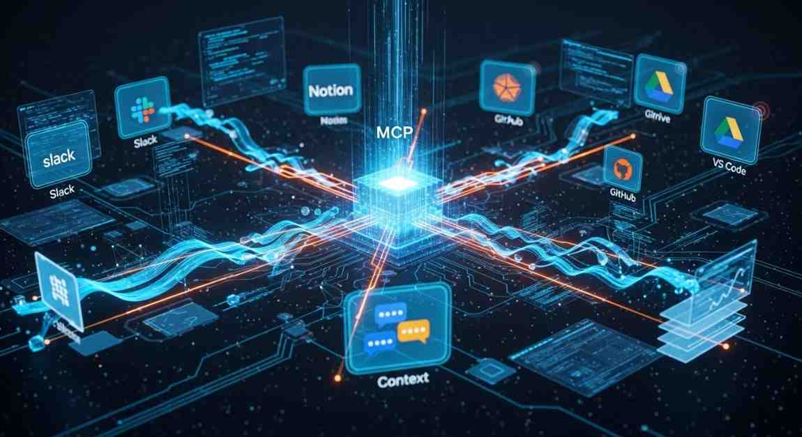
Instead of every AI tool building integrations with every service, Model Context Protocol introduces a standardized protocol. GitHub builds one MCP server that any AI tool can connect to. Google Drive builds one MCP server. Slack builds one MCP server. 

Now the equation changes from N×M to N+M integrations. A massive reduction in complexity. 

The network effects are powerful: More AI chatbots supporting Model Context Protocol makes it more valuable for services to build MCP servers. More MCP servers available makes it more valuable for AI tools to support MCP. More adoption leads to more standardization, which creates more ecosystem value. Not supporting MCP means being cut off from a rapidly growing ecosystem. 

Explore how LLM-agents convert language models into action-capable tools and why that matters.

Understanding Model Context Protocol (MCP) Architecture 

The Simplest Version 

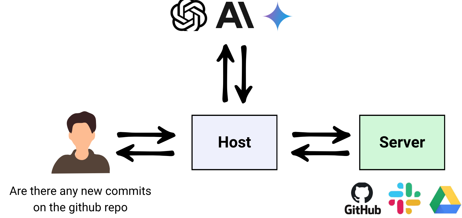
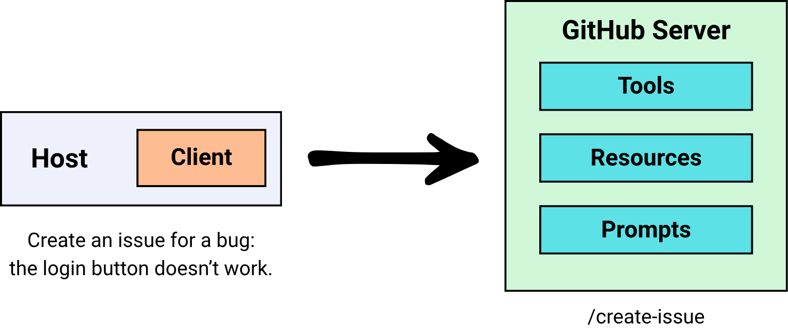
At its core, MCP has three components: 

1. Host/Client: The AI application (like Claude Desktop, ChatGPT, or a custom AI assistant) 
2. MCP Server: A program that provides access to specific services or data 
3. Communication Protocol: The standardized way they talk to each other 

Here’s a simple example: You ask Claude, “Are there any new commits on the GitHub repo?” Claude (the Host) sends a request to the GitHub MCP Server, which fetches the information and sends it back. 

Key Benefits of This Architecture 

• Decoupling: The Host doesn’t need to know how GitHub’s API works. The MCP Server handles all the complexity. 
• Safety: The Server can implement security controls, rate limiting, and access policies independent of the Host. 
• Scalability: Multiple Hosts can connect to the same Server without modification. 
• Parallelism: Hosts can query multiple Servers simultaneously. 

Model Context Protocol (MCP) Primitives: The Building Blocks 

Model Context Protocol defines three core primitives, things a server can offer to a host: 

1. Tools

Tools are actions the AI can ask the server to perform. Think of them as functions the AI can call. 

Examples: 

• create_github_issue: Create a new issue in a repository 
• send_email: Send an email through Gmail 
• search_documents: Search through Google Drive files 

2. Resources

Resources are structured data sources that the AI can read. These provide context without requiring active queries. 

Examples: 

• Current contents of a file 
• List of recent commits 
• Database schema 
• User profile information 

3. Prompts

Prompts are predefined templates or instructions that help shape the AI’s behavior for specific tasks. 

For example, instead of the user saying, “Create an issue for a bug: the login button doesn’t work” (which is too vague), an MCP Server can provide a structured prompt template: 

This ensures consistency and quality in how the AI formulates requests. 

The Data Layer: JSON-RPC 2.0 

The data layer is the language and grammar that everyone in the Model Context Protocol ecosystem agrees upon to communicate. MCP uses JSON-RPC 2.0 as its foundation. 

What Is JSON-RPC? 

JSON-RPC stands for JavaScript Object Notation – Remote Procedure Call. An RPC allows a program to execute a function on another computer as if it were local, hiding the complexity of network communication. Instead of writing add(2, 3) locally, you send a request to a server saying “please run add with parameters 2 and 3.” 

JSON-RPC combines remote procedure calls with the simplicity of JSON, creating a standardized format for requests and responses. 

Why JSON-RPC for Model Context Protocol? 

• Bi-directional communication: Both client and server can initiate requests 
• Transport-agnostic: Works over different connection types 
• Supports batching: Multiple requests in one message 
• Supports notifications: One-way messages that don’t require responses 
• Lightweight: Minimal overhead 

Request Structure 

  

Response Structure 

  

The Transport Layer: Moving Messages 

The transport layer is the mechanism that physically moves JSON-RPC messages between the client and server. Model Context Protocol supports two main types of servers, each with its own transport: 

Local Servers: STDIO 

STDIO (Standard Input/Output) is used for servers running on your own computer. 

Every program has built-in streams: 

• stdin: Input the program reads 
• stdout: Output the program writes 

In Model Context Protocol, the host launches the server as a subprocess and uses these streams for communication. The host writes JSON-RPC messages to the server’s stdin, and the server writes responses to its stdout. 

Benefits: 

• Fast: Data passes directly between processes 
• Secure: No open network ports; communication is only local 
• Simple: Every language supports stdin/stdout; no extra libraries required 

Discover the communication protocols that enable multiple autonomous agents to coordinate and function at scale.

Remote Servers: HTTP + SSE 

For servers running elsewhere on the network, Model Context Protocol uses HTTP with Server-Sent Events (SSE). 

The host sends JSON-RPC requests as HTTP POST requests with JSON payloads. The transport supports standard HTTP authentication methods like API keys. 

SSE extends HTTP to allow the server to send multiple messages to the client over a single open connection. Instead of one large JSON blob, the server can stream chunks of data as they become available. This is ideal for long-running tasks or incremental updates. 

The Model Context Protocol Lifecycle 

The Model Context Protocol lifecycle describes the complete sequence of steps governing how a host and server establish, use, and end a connection. 

Phase 1: Initialization 

Initialization must be the first interaction between client and server. Its purpose is to establish protocol version compatibility and exchange capabilities. 

Step 1 – Client Initialize Request: The client sends an initialize request containing its implementation info, MCP protocol version, and capabilities. 

Step 2 – Server Response: The server responds with its own implementation info, protocol version, and capabilities. 

Step 3 – Initialized Notification: After successful initialization, the client must send an initialized notification to indicate it’s ready for normal operations. 

Important Rules: 

• The client should not send requests (except pings) before the server responds to initialization 

• The server should not send requests (except pings and logging) before receiving the initialized notification 

Version Negotiation 

Both sides declare which protocol versions they support. They then agree to use the highest mutually supported version. If no common version exists, the connection fails immediately. 

Capability Negotiation 

Client and server capabilities establish which protocol features will be available during the session. Each side declares what it can do, and only mutually supported features can be used. 

For example, if a client doesn’t declare support for prompts, the server won’t offer any prompt templates. 

Phase 2: Operation 

During the operation phase, the client and server exchange messages according to negotiated capabilities. 

Capability Discovery: The client can ask “what tools do you have?” or “what resources can you provide?” 

Tool Calling: The client can invoke tools, and the server executes them and returns results. 

Throughout this phase, both sides must respect the negotiated protocol version and only use capabilities that were successfully negotiated. 

Discover key design patterns behind AI agents built on LLMs and learn how to apply them effectively.

Phase 3: Shutdown 

One side (typically the client) initiates shutdown. No special JSON-RPC shutdown message is defined—the transport layer signals termination. 

For STDIO: The client closes the input stream to the server process, waits for the server to exit, and sends termination signals (SIGTERM, then SIGKILL if necessary) if the server doesn’t exit gracefully. 

For HTTP: The client closes HTTP connections, or the server may close from its side. The client must detect dropped connections and handle them appropriately. 

Special Cases in MCP 

1. Pings 

Ping is a lightweight request/response method to check whether the other side is still alive and the connection is responsive. 

When is it used? 

• Before full initialization to check if the other side is up 

• Periodically during inactivity to maintain the connection 

• To prevent connections from being dropped by the OS, proxies, or firewalls 

2. Error Handling 

MCP inherits JSON-RPC’s standard error object format. 

Common causes of errors: 

• Unsupported or mismatched protocol version 

• Calling a method for a capability that wasn’t negotiated 

• Invalid arguments to a tool 

• Internal server failure during processing 

• Timeout exceeded leading to request cancellation 

• Malformed JSON-RPC messages 

Error Object Structure: 

  

3. Timeout and Cancellation 

Timeouts protect against unresponsive servers and ensure resources aren’t held indefinitely. 

The client sets a per-request timeout (for example, 30 seconds). If the deadline passes with no result, the client triggers a timeout and sends a cancellation notification to tell the server to stop processing. 

4. Progress Notifications 

For long-running requests, the server can send progress updates to let the client know work is continuing. 

The client includes a progressToken in the request metadata. The server then sends progress notifications while working, keeping the user informed instead of leaving them wondering if anything is happening. 

Getting Started with Model Context Protocol

Using Claude Desktop 

The easiest way to experience Model Context Protocol is through Claude Desktop, which has built-in support for MCP servers. 

There are two types of connections you can set up: 

1. Local Servers: Configure MCP servers that run on your machine using a configuration file. These use STDIO transport and are perfect for accessing local resources, development tools, or services that require local execution.
2. Remote Servers: Connect to MCP servers hosted elsewhere using HTTP/SSE transport. These are ideal for cloud services and APIs.

Configuration vs. Connectors 

Configuration File Method: You manually edit a configuration file to specify which MCP servers Claude should connect to. This gives you complete control and allows you to use any MCP server, whether it’s official or community-built. 

Connectors: Built-in features that link Claude to MCP servers automatically, without manual setup. Think of Connectors as the “App Store” for MCP servers—user-friendly, click-based, and pre-curated. 

Connectors are officially built, hosted, and maintained by Anthropic. They come with OAuth login flows, managed security, rate limits, and guaranteed stability. Most Claude Desktop users are non-technical end-users who just want Claude to “talk” to their apps (Notion, Google Drive, GitHub, Slack) without running servers or editing JSON. 

Why Not Use Connectors Always? 

Model Context Protocol is an open standard designed so anyone can write a server. If every MCP server were required to be a Connector, Anthropic would need to review, host, and secure every possible server. This approach does not scale. 

Forcing everything through Connectors would close the ecosystem and create dependency on Anthropic to approve or publish servers. The configuration file method keeps Model Context Protocol truly open while Connectors provide convenience for mainstream users. 

Building Your Own MCP Server 

The beauty of Model Context Protocol is that anyone can build a server. Anthropic provides SDKs for both clients and servers, making development straightforward. 

Key considerations when building a server: 

• Choose your primitives: Will you expose tools, resources, prompts, or a combination?

• Implement security: Add authentication, rate limiting, and access controls

• Handle errors gracefully: Provide clear error messages and proper status codes

• Support the lifecycle: Properly implement initialization, operation, and shutdown phases

• Document you capabilities: Make it clear what your server can do

Explore the internal mechanics of LLMs so you can better understand what agents are building on.

The Future of Model Context Protocol

Model Context Protocol represents a fundamental shift in how AI systems integrate with the digital world. Instead of every AI tool building its own integrations with every service, we now have a standardized protocol that dramatically reduces complexity. 

The network effects are already building momentum. As more AI platforms support Model Context Protocol and more services build MCP servers, the ecosystem becomes increasingly valuable for everyone. Organizations that don’t support Model Context Protocol risk being left out of this growing interconnected AI ecosystem. 

For developers, Model Context Protocol opens up possibilities to create servers that work across all MCP-compatible AI platforms. For users, it means AI assistants that can seamlessly access and interact with all your tools and services through a unified interface. 

We’re moving from a world of fragmented AI assistants to one where AI truly understands your entire work context, not because it’s been trained on your data, but because it can dynamically access what it needs through standardized, secure protocols. 

Conclusion 

Model Context Protocol solves one of the most pressing challenges in the AI era: enabling AI systems to access the context they need without creating an integration nightmare. 

By understanding Model Context Protocol’s architecture, from its primitives and data layer to its transport mechanisms and lifecycle, you’re now equipped to both use existing MCP servers and build your own. Whether you’re a developer creating integrations, a business leader evaluating AI tools, or a power user wanting to maximize your AI assistant’s capabilities, Model Context Protocol is the standard that will shape how AI systems connect to the world. 

The age of fragmented AI tools is ending. The age of unified, context-aware AI assistance is just beginning. 

Ready to build the next generation of agentic AI?
Explore our Large Language Models Bootcamp and Agentic AI Bootcamp for hands-on learning and expert guidance.

Think about how much time we spend on small, repetitive tasks every day. Answering emails, updating spreadsheets, saving files, or copying data from one app to another. Each task might take only a few minutes, but together they consume hours of our week. 

Now imagine if these tasks could take care of themselves. Imagine if your email could be sorted, important notes stored, and reminders sent to you automatically, all without you touching a button. That is the power of automation. 

And when we add AI agents into the mix, things become even more exciting. Instead of just following rigid rules, AI can help automations understand, reason, and adapt. 

In this guide, we’ll walk through what automation is, how AI agents expand its possibilities, which tools you can use to get started, and a simple hands-on example using n8n to tie it all together. 

Understand how AI agents go beyond rules and act autonomously.

What is Automation? 

At its simplest, automation is about letting software handle routine tasks, so you don’t have to. Think of it as a set of “if this, then that” instructions. 

• If someone fills out a form, add their details to a spreadsheet. 

• If an order is placed, send a thank-you email. 

• If a file is uploaded, back it up to the cloud. 

These are straightforward rules, but they save time and prevent mistakes. Automation takes away the repetitive work, leaving you free to focus on more important things. 

How AI Agents Make Automations Smarter 

While traditional automation is powerful, it has limits. It can only follow rules you give it. What happens when a task requires judgment, creativity, or understanding context? 

This is where AI agents come in. Unlike simple rule-based systems, AI agents can: 

• Read and understand text, not just keywords. 

• Summarize documents or emails. 

• Categorize information based on meaning, not rigid filters. 

• Decide the next best action depending on the situation. 

In other words, AI agents give automation the ability to think. They don’t just follow instructions; they make decisions along the way. 

Here’s a simple illustration that shows how automation runs on strict rules, while AI agents can adjust and choose their own path. 

Tools That Make Automation Possible 

The good news is you don’t need to be a programmer to build these automations. Today, several tools make it simple for anyone to connect apps, add AI, and create workflows. Let’s look at a few popular ones: 

n8n 

n8n is an open-source automation tool that gives you control and flexibility. It has a drag-and-drop interface where you connect apps like Gmail, Slack, Notion, and even AI services. You can host it yourself, which makes it a great option if you care about data privacy. 

Zapier 

Zapier is one of the most widely used automation platforms. It connects with thousands of apps, so you can quickly build workflows without technical knowledge. For beginners, it’s one of the easiest ways to start automating tasks. 

Make (formerly Integromat) 

Make also offers a visual way to build automation, but it shines when workflows get more complex. If you want detailed control over each step in a process, Make is worth exploring. 

Turn insights into action by automating your data flow from Azure Synapse to SharePoint Excel.

AI-Centered Platforms 

Some tools focus directly on building AI-powered workflows: 

• Flowise lets you create conversational AI agents with a visual editor. 

• Relevance AI helps automate data-heavy tasks with AI models at the core. 

These platforms are designed for scenarios where AI is not just an add-on, but the main driver. 

Discover tools that empower developers to create intelligent, autonomous agents

Examples of Automation with AI 

To see how automation and AI come together, let’s look at a few practical scenarios. 

1. Smarter Email Management

Imagine receiving dozens of emails every day. Some are urgent, others less important, but all need to be read. An automation can help: 

• New emails are collected automatically. 

• An AI agent summarizes the content in plain language. 

• Urgent ones are flagged and sent as a short notification. 

This means you no longer scroll through endless messages. Instead, you get a quick overview that saves time and helps you focus. 

2. Content Idea Generation

Staying up to date with trends can be tiring. An automation can gather topics from sources like Reddit or Twitter, send them to an AI model for analysis, and produce blog or video outline ideas. The outlines are stored in a document tool, ready for review. 

What once took hours of manual research and note-taking is reduced to a few clicks. 

Email Summarization Workflow in n8n 

Now, let’s make this more concrete with a simple workflow in n8n. Suppose the goal is to summarize incoming emails and send the summaries to Slack. Here’s how that might look: 

1. Trigger Node: Start with the Gmail node, set it to trigger whenever a new email arrives. 
2. AI Node: Add the Google Gemini node. Connect it to the Gmail node and configure it to summarize the email body text. 
3. Messaging Node: Add a Slack node. Send the summary as a message to a specific channel or directly to yourself. 
4. Run the Workflow: Each time an email comes in, the workflow triggers automatically, generates a summary, and posts it to Slack. 

With just a few nodes, you now have a smart automation that saves time and improves focus. 

Here’s how the workflow looks inside n8n. The flow clearly shows how an email moves through each step until the summary reaches Slack. 

This is just one simple example of what a workflow can do. With n8n and AI, you can design many more automations that fit different needs. 

Understand how LangChain enhances AI agent capabilities for complex workflows.

Why Automation and AI Matter Together 

When combined, automation and AI deliver more than convenience. They bring real advantages: 

• Time Savings: Repetitive tasks disappear from your to-do list. 

• Consistency: Processes run the same way every time, reducing errors. 

• Scalability: You can handle more work without more effort. 

• Smarter Workflows: AI helps with understanding and decision-making. 

This isn’t about replacing humans. It’s about removing the busy work so we can focus on tasks that need creativity, empathy, and strategy. 

How to Start 

Getting started doesn’t need to feel overwhelming. Here’s a simple approach: 

1. Identify a small repetitive task you do often. 
2. Pick a tool like Zapier, n8n, or Make. 
3. Build a simple workflow, like moving email attachments to cloud storage. 
4. Once comfortable, add an AI step, such as summarizing text or categorizing feedback. 

The key is to start small, see the benefit, and then expand step by step. 

Explore how memory integration transforms AI agents from reactive to proactive systems.

Final Thoughts 

Automation alone saves time, but with AI agents it becomes transformative. You move from rules that repeat tasks to intelligent systems that adapt and make decisions. 

Whether you choose n8n, Zapier, Make, or an AI-focused tool like Flowise, the possibilities are wide open. By starting small and growing gradually, you can turn everyday processes into smart workflows that work for you. 

The future of work is not just about doing things faster, but about working smarter. Automation and AI agents are tools that bring that future within reach, starting today. 

Ready to build the next generation of agentic AI?
Explore our Large Language Models Bootcamp and Agentic AI Bootcamp for hands-on learning and expert guidance.

In the vast forest of machine learning algorithms, one algorithm stands tall like a sturdy tree – Random Forest. It’s an ensemble learning method that’s both powerful and flexible, widely used for classification and regression tasks.

But what makes the random forest algorithm so effective? How does it work?

In this blog, we’ll explore the inner workings of Random Forest, its advantages, limitations, and practical applications. 

What is a Random Forest Algorithm? 

Imagine a dense forest with numerous trees, each offering a different path to follow. Random Forest Algorithm is like that: an ensemble of decision trees working together to make more accurate predictions.

By combining the results of multiple trees, the algorithm improves the overall model performance, reducing errors and variance.

 

 

 

Why the Name ‘Random Forest’? 

The name “Random Forest” comes from the combination of two key concepts: randomness and forests. The “random” part refers to the random selection of data samples and features during the construction of each tree, while the “forest” part refers to the ensemble of decision trees.

This randomness is what makes the algorithm robust and less prone to overfitting. 

Common Use Cases of Random Forest Algorithm

Random Forest Algorithm is highly versatile and is used in various applications such as: 

• Classification: Spam detection, disease prediction, customer segmentation. 

• Regression: Predicting stock prices, house values, and customer lifetime value. 

 

Also learn about Linear vs Logistic regression

 

Understanding the Basics 

Before diving into Random Forest, let’s quickly revisit the concept of Decision Trees. 

Decision Trees Recap 

A decision tree is a flowchart-like structure where internal nodes represent decisions based on features, branches represent the outcomes of these decisions, and leaf nodes represent final predictions. While decision trees are easy to understand and interpret, they can be prone to overfitting, especially when the tree is deep and complex.

 

 

Key Concepts in Random Forest 

• Ensemble Learning: This technique combines multiple models to improve performance. Random Forest is an example of ensemble learning where multiple decision trees work together to produce a more accurate and stable prediction. 

 

Read in detail about ensemble methods in machine learning

 

• Bagging (Bootstrap Aggregating): In Random Forest, the algorithm creates multiple subsets of the original dataset by sampling with replacement (bootstrapping). Each tree is trained on a different subset, which helps in reducing variance and preventing overfitting. 

• Feature Randomness: During the construction of each tree, Random Forest randomly selects a subset of features to consider at each split. This ensures that the trees are diverse and reduces the likelihood that a few strong predictors dominate the model.

 

 

How Does Random Forest Work? 

Let’s break down the process into two main phases: training and prediction. 

Training Phase 

• Creating Bootstrapped Datasets: The algorithm starts by creating multiple bootstrapped datasets by randomly sampling the original data with replacement. This means some data points may be repeated, while others may be left out. 

• Building Multiple Decision Trees: For each bootstrapped dataset, a decision tree is constructed. However, instead of considering all features at each split, the algorithm randomly selects a subset of features. This randomness ensures that the trees are different from each other, leading to a more generalized model. 

Prediction Phase 

• Voting in Classification: When it’s time to make predictions, each tree in the forest casts a vote for the class label. The final prediction is determined by the majority vote among the trees. 

• Averaging in Regression: For regression tasks, instead of voting, the predictions from all the trees are averaged to get the result.

 

Another interesting read: Sustainability Data and Machine Learning

 

Advantages of Random Forest 

Random Forest is popular for good reasons. Some of these include:

High Accuracy 

By aggregating the predictions of multiple trees, Random Forest often achieves higher accuracy than individual decision trees. The ensemble approach reduces the impact of noisy data and avoids overfitting, making the model more reliable. 

Robustness to Overfitting 

Overfitting occurs when a model performs well on the training data but poorly on unseen data. Random Forest combats overfitting by averaging the predictions of multiple trees, each trained on different parts of the data. This ensemble approach helps the model generalize better. 

Handles Missing Data 

Random Forest can handle missing values naturally by using the split with the majority of the data and by averaging the outputs from trees trained on different parts of the data. 

Feature Importance 

One of the perks of Random Forest is its ability to measure the importance of each feature in making predictions. This is done by evaluating the impact of each feature on the model’s performance, providing insights into which features are most influential.

 

 

Limitations of Random Forest 

While Random Forest is a powerful tool, it’s not without its drawbacks. A few limitations associated with random forests are:

Computational Cost 

Training multiple decision trees can be computationally expensive, especially with large datasets and a high number of trees. The algorithm’s complexity increases with the number of trees and the depth of each tree, leading to longer training times. 

Interpretability 

While decision trees are easy to interpret, Random Forest, being an ensemble of many trees, is more complex and harder to interpret. The lack of transparency can be a disadvantage in situations where model interpretability is crucial. 

Bias-Variance Trade-off 

Random Forest does a good job managing the bias-variance trade-off, but it’s not immune to it. If not carefully tuned, the model can still suffer from bias or variance issues, though typically less so than a single decision tree. 

Hyperparameter Tuning in Random Forest

While we understand the benefits and limitations of Random Forest, let’s take a deeper look into working with the algorithm. Understanding and working with relevant hyperparameters is a crucial part of the process.

It is an important aspect because tuning the hyperparameters of a Random Forest can significantly impact its performance. Here are some key hyperparameters to consider:

Master hyperparameter tuning for machine learning models

 

Key Hyperparameters 

• Number of Trees (n_estimators): The number of trees in the forest. Increasing this generally improves performance but with diminishing returns and increased computational cost. 

• Maximum Depth (max_depth): The maximum depth of each tree. Limiting the depth can help prevent overfitting. 

• Number of Features (max_features): The number of features to consider when looking for the best split. Lower values increase diversity among trees but can also lead to underfitting. 

Techniques for Tuning 

• Grid Search: This exhaustive search technique tries every combination of hyperparameters within a specified range to find the best combination. While thorough, it can be time-consuming. 

• Random Search: Instead of trying every combination, Random Search randomly selects combinations of hyperparameters. It’s faster than Grid Search and often finds good results with less computational effort. 

• Cross-Validation: Cross-validation is essential in hyperparameter tuning. It splits the data into several subsets and uses different combinations for training and validation, ensuring that the model’s performance is not dependent on a specific subset of data.

Practical Implementation 

To understand how Random Forest works in practice, let’s look at a step-by-step implementation using Python. 

Setting Up the Environment 

You’ll need the following Python libraries: scikit-learn for the Random Forest implementation, pandas for data handling, and numpy for numerical operations.

 

 

Example Dataset 

For this example, we’ll use the famous Iris dataset, a simple yet effective dataset for demonstrating classification algorithms. 

Step-by-Step Code Walkthrough 

• Data Preprocessing: Start by loading the data and handling any missing values, though the Iris dataset is clean and ready to use.

 

 

• Training the Random Forest Model: Instantiate the Random Forest classifier and fit it to the training data. 

 

 

• Evaluating the Model: Use the test data to evaluate the model’s performance.

 

 

• Hyperparameter Tuning: Use Grid Search or Random Search to find the optimal hyperparameters.

 

 

Comparing Random Forest with Other Algorithms 

Random Forest vs. Decision Trees 

While a single decision tree is easy to interpret, it’s prone to overfitting, especially with complex data. Random Forest reduces overfitting by averaging the predictions of multiple trees, leading to better generalization.

 

Explore the boosting algorithms used to enhance ML model accuracy

 

Random Forest vs. Gradient Boosting 

Both are ensemble methods, but they differ in approach. Random Forest builds trees independently, while Gradient Boosting builds trees sequentially, where each tree corrects the errors of the previous one. Gradient Boosting often achieves better accuracy but at the cost of higher computational complexity and longer training times. 

Random Forest vs. Support Vector Machines (SVM) 

SVMs are powerful for high-dimensional data, especially when the number of features exceeds the number of samples. However, SVMs are less interpretable and more sensitive to parameter tuning compared to Random Forest. Random Forest tends to be more robust and easier to use out of the box.

 

 

Explore the Impact of Random Forest Algorithm

Random Forest is a powerful and versatile algorithm, capable of handling complex datasets with high accuracy. Its ensemble nature makes it robust against overfitting and capable of providing valuable insights into feature importance. 

As you venture into the world of machine learning, remember that a well-tuned Random Forest can be the key to unlocking insights hidden deep within your data. Keep experimenting, stay curious, and let your models grow as robust as the forest itself!

Machine learning (ML) is a field where both art and science converge to create models that can predict outcomes based on data. One of the most effective strategies employed in ML to enhance model performance is ensemble methods.

Rather than relying on a single model, ensemble methods combine multiple models to produce better results. This approach can significantly boost accuracy, reduce overfitting, and improve generalization. 

In this blog, we’ll explore various ensemble techniques, their working principles, and their applications in real-world scenarios.

 

 

What Are Ensemble Methods?

Ensemble methods are techniques that create multiple models and then combine them to produce a more accurate and robust final prediction. The idea is that by aggregating the predictions of several base models, the ensemble can capture the strengths of each individual model while mitigating their weaknesses.

 

Also explore this: Azure Machine Learning in 5 Simple Steps

 

Why Use Ensemble Methods? 

Ensemble methods are used to improve the robustness and generalization of machine learning models by combining the predictions of multiple models. This can reduce overfitting and improve performance on unseen data.

 

Read more Gini Index and Entropy

 

Types of Ensemble Methods 

There are three primary types of ensemble methods: Bagging, Boosting, and Stacking. 

Bagging (Bootstrap Aggregating) 

Bagging involves creating multiple subsets of the original dataset using bootstrap sampling (random sampling with replacement). Each subset is used to train a different model, typically of the same type, such as decision trees. The final prediction is made by averaging (for regression) or voting (for classification) the predictions of all models.

 

 

How Bagging Works: 

• Bootstrap Sampling: Create multiple subsets from the original dataset by sampling with replacement. 

• Model Training: Train a separate model on each subset. 

• Aggregation: Combine the predictions of all models by averaging (regression) or majority voting (classification). 

Random Forest 

Random Forest is a popular bagging method where multiple decision trees are trained on different subsets of the data, and their predictions are averaged to get the final result. 

Boosting 

Boosting is a sequential ensemble method where models are trained one after another, each new model focusing on the errors made by the previous models. The final prediction is a weighted sum of the individual model’s predictions.

 

 

How Boosting Works:

• Initialize Weights: Start with equal weights for all data points. 

• Sequential Training: Train a model and adjust weights to focus more on misclassified instances. 

• Aggregation: Combine the predictions of all models using a weighted sum. 

AdaBoost (Adaptive Boosting)  

It assigns weights to each instance, with higher weights given to misclassified instances. Subsequent models focus on these hard-to-predict instances, gradually improving the overall performance. 

 

You might also like: ML using Python in Cloud

 

Gradient Boosting 

It builds models sequentially, where each new model tries to minimize the residual errors of the combined ensemble of previous models using gradient descent. 

XGBoost (Extreme Gradient Boosting) 

An optimized version of Gradient Boosting, known for its speed and performance, is often used in competitions and real-world applications. 

Stacking 

Stacking, or stacked generalization, involves training multiple base models and then using their predictions as inputs to a higher-level meta-model. This meta-model is responsible for making the final prediction.

 

 

How Stacking Works: 

• Base Model Training: Train multiple base models on the training data. 

• Meta-Model Training: Use the predictions of the base models as features to train a meta-model. 

Example: 

A typical stacking ensemble might use logistic regression as the meta-model and decision trees, SVMs, and KNNs as base models.

 

 

Benefits of Ensemble Methods

Improved Accuracy 

By combining multiple models, ensemble methods can significantly enhance prediction accuracy. 

Robustness 

Ensemble models are less sensitive to the peculiarities of a particular dataset, making them more robust and reliable. 

Reduction of Overfitting 

By averaging the predictions of multiple models, ensemble methods reduce the risk of overfitting, especially in high-variance models like decision trees. 

Versatility 

Ensemble methods can be applied to various types of data and problems, from classification to regression tasks. 

Applications of Ensemble Methods 

Ensemble methods have been successfully applied in various domains, including: 

• Healthcare: Improving the accuracy of disease diagnosis by combining different predictive models.
• Finance: Enhancing stock price prediction by aggregating multiple financial models.
• Computer Vision: Boosting the performance of image classification tasks with ensembles of CNNs.

 

Here’s a list of the top 7 books to master your learning on computer vision

 

Implementing Random Forest in Python 

Now let’s walk through the implementation of a Random Forest classifier in Python using the popular scikit-learn library. We’ll use the Iris dataset, a well-known dataset in the machine learning community, to demonstrate the steps involved in training and evaluating a Random Forest model. 

Explanation of the Code 

Import Necessary Libraries

 

We start by importing the necessary libraries. numpy is used for numerical operations, train_test_split for splitting the dataset, RandomForestClassifier for building the model, accuracy_score for evaluating the model, and load_iris to load the Iris dataset. 

Load the Iris Dataset

 

The Iris dataset is loaded using load_iris(). The dataset contains four features (sepal length, sepal width, petal length, and petal width) and three classes (Iris setosa, Iris versicolor, and Iris virginica). 

Split the Dataset

 

We split the dataset into training and testing sets using train_test_split(). Here, 30% of the data is used for testing, and the rest is used for training. The random_state parameter ensures the reproducibility of the results. 

Initialize the RandomForestClassifier

 

We create an instance of the RandomForestClassifier with 100 decision trees (n_estimators=100). The random_state parameter ensures that the results are reproducible. 

Train the Model

 

We train the Random Forest classifier on the training data using the fit() method. 

Make Predictions

 

After training, we use the predict() method to make predictions on the testing data. 

Evaluate the Model

 

Finally, we evaluate the model’s performance by calculating the accuracy using the accuracy_score() function. The accuracy score is printed to two decimal places. 

Output Analysis 

When you run this code, you should see an output similar to:

 

 

This output indicates that the Random Forest classifier achieved 100% accuracy on the testing set. This high accuracy is expected for the Iris dataset, as it is relatively small and simple, making it easy for many models to achieve perfect or near-perfect performance.

In practice, the accuracy may vary depending on the complexity and nature of the dataset, but Random Forests are generally robust and reliable classifiers. 

By following this guided practice, you can see how straightforward it is to implement a Random Forest model in Python. This powerful ensemble method can be applied to various datasets and problems, offering significant improvements in predictive performance.

 

 

 

 

Summing it Up

To sum up, Ensemble methods are powerful tools in the machine learning toolkit, offering significant improvements in predictive performance and robustness. By understanding and applying techniques like bagging, boosting, and stacking, you can create models that are more accurate and reliable. 

Ensemble methods are not just theoretical constructs; they have practical applications in various fields. By leveraging the strengths of multiple models, you can tackle complex problems with greater confidence and precision.

Time series data, a continuous stream of measurements captured over time, is the lifeblood of countless fields. From stock market trends to weather patterns, it holds the key to understanding and predicting the future.

Traditionally, unraveling these insights required wading through complex statistical analysis and code. However, a new wave of technology is making waves: Large Language Models (LLMs) are revolutionizing how we analyze time series data, especially with the use of LangChain agents.

 

Explore LLM Guide

 

In this article, we will navigate the exciting world of LLM-based time series analysis. We will explore how LLMs can be used to unearth hidden patterns in your data, forecast future trends, and answer your most pressing questions about time series data using plain English.

 

 

We will see how to integrate Langchain’s Pandas Agent, a powerful LLM tool, into your existing workflow for seamless exploration. 

Uncover Hidden Trends with LLMs 

LLMs are powerful AI models trained on massive amounts of text data. They excel at understanding and generating human language. But their capabilities extend far beyond just words. Researchers are now unlocking their potential for time series analysis by bridging the gap between numerical data and natural language. 

 

Understand How LLM Development is making Chatbots Smarter.

Here’s how LLMs are transforming the game: 

• Natural Language Prompts: Imagine asking questions about your data like, “Is there a correlation between ice cream sales and temperature?” LLMs can be prompted in natural language, deciphering your intent, and performing the necessary analysis on the underlying time series data. 
• Pattern Recognition: LLMs excel at identifying patterns in language. This ability translates to time series data as well. They can uncover hidden trends, periodicities, and seasonality within the data stream. 
• Uncertainty Quantification: Forecasting the future is inherently uncertain. LLMs can go beyond just providing point predictions. They can estimate the likelihood of different outcomes, giving you a more holistic picture of potential future scenarios.

LLM Applications Across Various Industries 

While LLM-based time series analysis is still evolving, it holds immense potential for various applications: 

• Financial analysis: Analyze market trends, predict stock prices, and identify potential risks with greater accuracy. 

 

Learn more about LLM Finance

 

• Supply chain management: Forecast demand fluctuations, optimize inventory levels, and prevent stockouts. 
• Scientific discovery: Uncover hidden patterns in environmental data, predict weather patterns, and accelerate scientific research. 
• Anomaly detection: Identify unusual spikes or dips in data streams, pinpointing potential equipment failures or fraudulent activities. 

 

 

LangChain Pandas Agent 

 

 

Lang Chain Pandas Agent is a Python library built on top of the popular Pandas library. It provides a comprehensive set of tools and functions specifically designed for data analysis. The agent simplifies the process of handling, manipulating, and visualizing time series data, making it an ideal choice for both beginners and experienced data analysts. 

 

Know more about LangChain and its Key Features

 

It exemplifies the power of LLMs for time series analysis. It acts as a bridge between these powerful language models and the widely used Panda’s library for data manipulation. Users can interact with their data using natural language commands, making complex analysis accessible to a wider audience. 

Key Features 

• Data Preprocessing: The agent offers various techniques for cleaning and preprocessing time series data, including handling missing values, removing outliers, and normalizing data. 
• Time-based Indexing: Lang Chain Pandas Agent allows users to easily set time-based indexes, enabling efficient slicing, filtering, and grouping of time series data. 
• Resampling and Aggregation: The agent provides functions for resampling time series data at different frequencies and aggregating data over specific time intervals. 
• Visualization: With built-in plotting capabilities, the agent allows users to create insightful visualizations such as line plots, scatter plots, and histograms to analyze time series data. 
• Statistical Analysis: Lang Chain Pandas Agent offers a wide range of statistical functions to calculate various metrics like mean, median, standard deviation, and more.

 

Read along to understand sentiment analysis in LLMs

 

Time Series Analysis with LangChain Pandas Agent 

Using LangChain Pandas Agent, we can perform a variety of time series analysis techniques, including: 

Trend Analysis: By applying techniques like moving averages and exponential smoothing, we can identify and analyze trends in time series data. 

 

Understand emerging AI and Machine Learning trends 

Seasonality Analysis: The agent provides tools to detect and analyze seasonal patterns within time series data, helping us understand recurring trends. 

Forecasting: With the help of advanced forecasting models like ARIMA and SARIMA, Lang Chain Pandas Agent enables us to make predictions based on historical time series data. 

LLMs in Action with LangChain Agents

Suppose you are using LangChain, a popular data analysis platform. LangChain’s Pandas Agent seamlessly integrates LLMs into your existing workflows. Here is how: 

1. Load your time series data: Simply upload your data into LangChain as you normally would. 
2. Engage the LLM: Activate LangChain’s Pandas Agent, your LLM-powered co-pilot. 
3. Ask away: Fire away your questions in plain English. “What factors are most likely to influence next quarter’s sales?” or “Is there a seasonal pattern in customer churn?” The LLM will analyze your data and deliver clear, concise answers. 

 

Learn to build custom chatbots using LangChain

 

Now Let’s explore Tesla’s stock performance over the past year and demonstrate how Language Models (LLMs) can be utilized for data analysis and unveil valuable insights into market trends.

To begin, we download the dataset and import it into our code editor using the following snippet:

 

 

Dataset Preview

Below are the first five rows of our dataset

 

 

Next, let’s install and import important libraries from LangChain that are instrumental in data analysis.

 

 

Following that, we will create a LangChain Pandas DataFrame agent utilizing OpenAI’s API.

 

With just these few lines of code executed, your LLM-based agent is now primed to extract valuable insights using simple language commands.

Initial Understanding of Data

Prompt

 

 

Explanation

The analysis of Tesla’s closing stock prices reveals that the average closing price was $217.16. There was a standard deviation of $37.73, indicating some variation in the daily closing prices. The minimum closing price was $142.05, while the maximum reached $293.34.

This comprehensive overview offers insights into the distribution and fluctuation of Tesla’s stock prices during the period analyzed.

Prompt

 

 

Explanation

The daily change in Tesla’s closing stock price is calculated, providing valuable insights into its day-to-day fluctuations. The average daily change, computed at 0.0618, signifies the typical amount by which Tesla’s closing stock price varied over the specified period.

This metric offers investors and analysts a clear understanding of the level of volatility or stability exhibited by Tesla’s stock daily, aiding in informed decision-making and risk assessment strategies.

Detecting Anomalies

Prompt

 

 

Explanation

In the realm of anomaly detection within financial data, the absence of outliers in closing prices, as determined by the 1.5*IQR rule, is a notable finding. This suggests that within the dataset under examination, there are no extreme values that significantly deviate from the norm.

However, it is essential to underscore that while this statistical method provides a preliminary assessment, a comprehensive analysis should incorporate additional factors and context to conclusively ascertain the presence or absence of outliers.

This comprehensive approach ensures a more nuanced understanding of the data’s integrity and potential anomalies, thus aiding in informed decision-making processes within the financial domain.

Visualizing Data

Prompt

 

 

 

Explanation

The chart above depicts the daily closing price of Tesla’s stock plotted over the past year. The horizontal x-axis represents the dates, while the vertical y-axis shows the corresponding closing prices in USD. Each data point is connected by a line, allowing us to visualize trends and fluctuations in the stock price over time. 

By analyzing this chart, we can identify trends like upward or downward movements in Tesla’s stock price. Additionally, sudden spikes or dips might warrant further investigation into potential news or events impacting the stock market.

Forecasting

Prompt

 

 

Explanation

Even with historical data, predicting the future is a complex task for Large Language Models. Large language models excel at analyzing information and generating text, they cannot reliably forecast stock prices. The stock market is influenced by many unpredictable factors, making precise predictions beyond historical trends difficult.

The analysis reveals an average price of $217.16 with some variation, but for a more confident prediction of Tesla’s price next month, human experts and consideration of current events are crucial.

Key Findings

Prompt

 

 

Explanation

The generated natural language summary encapsulates the essential insights gleaned from the data analysis. It underscores the stock’s average price, revealing its range from $142.05 to $293.34. Notably, the analysis highlights the stock’s low volatility, a significant metric for investors gauging risk.

With a standard deviation of $37.73, it paints a picture of stability amidst market fluctuations. Furthermore, the observation that most price changes are minor, averaging just 0.26%, provides valuable context on the stock’s day-to-day movements.

This concise summary distills complex data into digestible nuggets, empowering readers to grasp key findings swiftly and make informed decisions.

Limitations and Considerations 

While LLMs offer significant advantages in time series analysis, it is essential to be aware of its limitations. These include the lack of domain-specific knowledge, sensitivity to input wording, biases in training data, and a limited understanding of context.

Data scientists must validate responses with domain expertise, frame questions carefully, and remain vigilant about biases and errors. 

• LLMs are most effective as a supplementary tool. They can be an asset for uncovering hidden patterns and providing context, but they should not be the sole basis for decisions, especially in critical areas like finance. 
• Combining LLMs with traditional time series models can be a powerful approach. This leverages the strengths of both methods – the ability of LLMs to handle complex relationships and the interpretability of traditional models. 

Overall, LLMs offer exciting possibilities for time series analysis, but it is important to be aware of their limitations and use them strategically alongside other tools for the best results.

 

 

Best Practices for Using LLMs in Time Series Analysis 

To effectively utilize LLMs like ChatGPT or Langchain in time series analysis, the following best practices are recommended: 

• Combine LLM’s insights with domain expertise to ensure accuracy and relevance. 
• Perform consistency checks by asking LMMs multiple variations of the same question. 
• Verify critical information and predictions with reliable external sources. 
• Use LLMs iteratively to generate ideas and hypotheses that can be refined with traditional methods. 
• Implement bias mitigation techniques to reduce the risk of biased responses. 
• Design clear prompts specifying the task and desired output. 
• Use a zero-shot approach for simpler tasks, and fine-tune for complex problems. 

 

 

LLMs: A Powerful Tool for Data Analytics

In summary, Large Language Models (LLMs) represent a significant shift in data analysis, offering an accessible avenue to obtain desired insights and narratives. The examples displayed highlight the power of adept prompting in unlocking valuable interpretations.

 

Read more on Bootcamps for LLM Training

 

However, this is merely the tip of the iceberg. With a deeper grasp of effective prompting strategies, users can unleash a wealth of analyses, comparisons, and visualizations.

Mastering the art of effective prompting allows individuals to navigate their data with the skill of seasoned analysts, all thanks to the transformative influence of LLMs.

 

Feature Engineering is a process of using domain knowledge to extract and transform features from raw data. These features can be used to improve the performance of Machine Learning Algorithms.

Feature Engineering encompasses a diverse array of techniques, including Feature Transformation, Feature Construction, Feature Selection, Feature Scaling, and Feature Extraction, each playing a crucial role in refining and optimizing the representation of data for machine learning tasks. 

In this blog, we will discuss one of the feature transformation techniques called feature scaling with examples and see how it will be the game changer for our machine learning model accuracy. 

 

 

 

In the world of data science and machine learning, feature transformation plays a crucial role in achieving accurate and reliable results. By manipulating the input features of a dataset, we can enhance their quality, extract meaningful information, and improve the performance of predictive models. Python, with its extensive libraries and tools, offers a streamlined and efficient process for simplifying feature scaling. 

What is Feature Scaling?

Feature scaling is a crucial step in the feature transformation process that ensures all features are on a similar scale. It is the process that normalizes the range of input columns and makes it useful for further visualization and machine learning model training. The figure below shows a quick representation of feature scaling techniques that we will discuss in this blog.

 

 

Why Feature Scaling is Important?

 

 

Feature scaling is important because of several factors:

• It improves the machine learning model’s accuracy
• It enhances the interpretability of data by transforming features on a common scale, without scaling, it is difficult to make comparisons of two features because of scale difference
• It speeds up the convergence in optimization algorithms like gradient descent algorithms
• It reduces the computational resources required for training the model
• For better accuracy, it is essential for the algorithms that rely on distance measures, such as K-nearest neighbors (KNN) and Support Vector Machines (SVM), to be sensitive to feature scales

Now let’s dive into some important methods of feature scaling and see how they impact data understanding and machine learning model performance.

 

Also learn about Machine Learning algorithms

 

Normalization

A feature scaling technique is often applied as part of data preparation for machine learning. The goal of normalization is to change the value of numeric columns in the dataset to use a common scale, without distorting differences in the range of values or losing any information.

Min-Max Scaler

The most commonly used normalization technique is min-max scaling, which transforms the features to a specific range, typically between 0 and 1. Scikit-learn has a built-in class available named MinMaxScaler that we can use directly for normalization. It involves subtracting the minimum value and dividing by the range of the feature using this formula.

 

 

Where,

X_i is the value we want to normalize.

X_max is the maximum value of the feature.

X_min is the minimum value of the feature.

In this transformation, the mean and standard deviation of the feature may behave differently. Our main focus in this normalization is on the minimum and maximum values. Outliers may disrupt our data pattern, so taking care of them is necessary.

 

Another interesting read: Building Predictive Models with Azure ML

 

Let’s take an example of a wine dataset that contains various ingredients of wine as features. We take two input features: the quantity of alcohol and malic acid and create a scatter plot as shown below.

 

 

When we create a scatter plot between alcohol and malic acid quantities, we can see that min-max scaling simply compresses our dataset into the range of zero to one, while keeping the distribution unchanged.

 

 

Standardization

Standardization is a feature scaling technique in which values of features are centered around the mean with unit variance. It is also called Z-Score Normalization. It subtracts the mean value of the feature and divides by the standard deviation (σ) of the feature using the formula:

 

 

Here we leverage a dataset on social network ads to gain a practical understanding of the concept. This dataset includes four input features: User ID, Gender, Age, and Salary. Based on this information, it determines whether the user made a purchase or not (where zero indicates not purchased, and one indicates purchased).

The first five rows of the dataset appear as follows:

 

 

In this example, we extract only two input features (Age and Salary) and use them to determine whether the output indicates a purchase or not as shown below.

 

Standard Scaler

We use Standard-Scaler from the Scikit-learn preprocessing module to standardize the input features for this feature scaling technique. The following code demonstrates this as shown.

 

 

We can see how our features look before and after standardization below.

 

 

Although it appears that the distribution changes after scaling, let’s visualize both distributions through a scatter plot.

 

 

So, when we visualize these distributions through plots, we observe that they remain the same as before. This indicates that scaling doesn’t alter the distribution; it simply centers it around the origin.

Now let’s see what happens when we create a density plot between Age and Estimated Salary with and without scaled features as shown below.

 

 

In the first plot, we can observe that we are unable to visualize the plot effectively and are not able to draw any conclusions or insights between age and estimated salary due to scale differences. However, in the second plot, we can visualize it and discern how age and estimated salary relate to each other.

 

You might also find this useful: Top Node.js Libraries for Machine Learning

 

This illustrates how scaling assists us by placing the features on similar scales. Note that this technique does not have any impact on outliers. So, if an outlier is present in the dataset, it remains as it is even after standardization. Therefore, we need to address outliers separately.

Model’s Performance Comparison

Now we use the logistic regression technique to predict whether a person will make a purchase after seeing an advertisement and observe how the model behaves with scaled features compared to without scaled features.

 

 

Here, we can observe a drastic improvement in our model accuracy when we apply the same algorithm to standardized features. Initially, our model accuracy is around 65.8%, and after standardization, it improves to 86.7% 

When Does It Matter?

Note that standardization does not always improve your model accuracy; its effectiveness depends on your dataset and the algorithms you are using. However, it can be very effective when you are working with multivariate analysis and similar methods, such as Principal Component Analysis (PCA), Support Vector Machine (SVM), K-means, Gradient Descent, Artificial Neural Networks (ANN), and K-nearest neighbors (KNN).

However, when you are working with algorithms like decision trees, random forest, Gradient Boosting (G-Boost), and (X-Boost), standardization may not have any impact on improving your model accuracy as these algorithms work on different principles and are not affected by differences in feature scales

To Sum It Up

We have covered standardization and normalization as two methods of feature scaling, including important techniques like Standard Scaler and Min-Max Scaler. These methods play a crucial role in preparing data for machine learning models, ensuring features are on a consistent scale. By standardizing or normalizing data, we enhance model performance and interpretability, paving the way for more accurate predictions and insights.