Transfer learning with Keras

This blog explains what transfer learning is, its benefits in image processing and how it’s applied. We will implement a model and train it for transfer learning using Keras.

What is transfer learning?

What if I told you that a network that classifies 10 different types of vehicles can provide useful knowledge for a classification problem with 3 different types of cars? This is called transfer learning – a method that uses pre-trained neural networks to solve a new, similar problem.

Over the years, people have been trying to produce different methods to train neural networks with small amounts of data. Those methods are used to generate more data for training. However, transfer learning provides an alternative by learning from existing architectures (trained on large datasets) and further training them for our new problem. This method reduces the training time and gives us a high accuracy in results for small datasets.

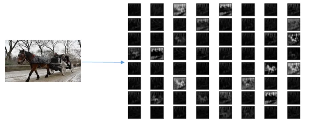
In image processing, the initial layers of the convolutional neural network (CNN) tend to learn basic features like the edges and boundaries in the image, while the deeper layers learn more complex features like tires of a vehicle, eyes of an animal, and various others describing the image in minute detail. The features learned by the initial layers are almost the same for different problems.

This is why, when using transfer learning, we only train the latter layers of the network. Since we only have to train the network for a few layers now, the learning is much faster, and we can achieve high accuracy even with a smaller dataset.

Getting started with the implementation

Now, let’s look at an example of applying transfer learning using the Keras library in Python. Keras provides us with many pre-trained networks by default that we can simply load and use for our tasks. For our implementation, we will use VGG19 as our reference pre-trained model. We want to train a model, so it can predict if the input image is a rickshaw (3-wheeler closed vehicle), tanga (horse/ donkey cart), or qingqi (3-wheeler open vehicle).

Data preparation

First, we will clone the dataset from GitHub, with images of rickshaw, qingqi, and tanga in our working directory using the following command.

!git clone https://github.com/MMFa666/VehicleDataset.git

Now, we will import all the libraries that we need for our task

'''
CV2 : Library to read image as matrix
numpy : Provides with mathematical toolkit
os : Helps reading files from their given paths
matplotlib : Used for plotting
'''
import cv2
import numpy as np
import os
import matplotlib.pyplot as plt
'''
keras : Provides us with the toolkit to build and train the model
'''
from tensorflow.keras.layers import Dense
from tensorflow.keras.optimizers import RMSprop
from tensorflow.keras import Model
from tensorflow import keras 

At this point, the images in the dataset are labeled as strings mentioning the names of the vehicle types. We need to convert the labels into quantitative formats by vectorizing each vehicle type.

In a vector with 3 values, each value can be either 1 or 0. The first value corresponds to the vehicle type ‘qingqi’, the second corresponds to vehicle type ‘rickshaw and the third to ‘tanga’. If the label is ‘qingqi’, the first value of the vector would be 1 and the rest would be 0 representing the unique vehicle type in the vector. These vectors are also called one-hot vectors because they have only one entry as ‘1’. It is an essential step for evaluating our model in the training process.

labels={}
labels['qingqi']=[1,0,0]
labels['rickshaw']=[0,1,0]
labels['tanga']=[0,0,1] 

Once we have vectorized, we will store the complete paths of all the images in a list so that they can be used to read the image as a matrix.

list_qingqi = [('/content/VehicleDataset/train/qingqi/' + i) for i in os.listdir('/content/VehicleDataset/train/qingqi')]
list_rickshaw =[('/content/VehicleDataset/train/rickshaw/' + i) for i in os.listdir('/content/VehicleDataset/train/rickshaw')]
list_tanga = [('/content/VehicleDataset/train/tanga/' + i) for i in os.listdir('/content/VehicleDataset/train/tanga')]
paths = list_qingqi + list_rickshaw + list_tanga 

Using the CV2 library, we will now read each image in the form of a matrix from its path. Moreover, each image is then re-sized to 224 x 224 which is the input shape for our network. These matrices are stored in a list named X.

Similarly, using the one-hot vectors we implemented above, we will make a list of Y labels that correspond to each image in X. The two lists, X and Y, are then randomly shuffled keeping the correspondence of X and Y unchanged. This prevents our model training to be biased towards any specific output label.

Finally, we use train_test_split function from sklearn to split our dataset into training and testing data.

perm = np.random.permutation(len(paths))
X = np.array([cv2.resize(cv2.imread(j) / 255, (224,224)) for j in paths])[perm]
Y = []
for i in range(len(paths)):
if i < len(list_qingqi):
Y.append(np.array(labels['qingqi']))
elif i < len(list_rickshaw):
Y.append(np.array(labels['rickshaw']))
else:
Y.append(np.array(labels['tanga']))
Y = np.array(Y)[perm]
from sklearn.model_selection import train_test_split
X_train, X_test, Y_train, Y_test = train_test_split(X, Y, test_size=0.1, random_state=42) 

Model set up

Step 1:

Keras library in Python provides us with various pre-trained networks by default. For our case, we would simply load the VGG19 model.

pretrained_model = keras.applications.vgg19.VGG19()

Step 2:

VGG19 was built to classify 19 different objects. However, we need the model to predict only 3 different objects. So, we initialize a new model and copy all the layers from VGG19 except the output layer having 19 nodes as in our case we only have 3 categories, hence, we create our own output layer with 3 outputs.

model = keras.Sequential()
for layer in pretrained_model.layers[:-1]:
model.add(layer)
model.add(Dense(3, activation = 'softmax'))

Step 3:

Since we do not want to train all the layers of the network but only the latter ones, we freeze the weights for the first 15 layers of the network and train only the last 10 layers.

for layer in model.layers:
layer.trainable = False

Training

Step 1

Define the hyper parameters that we need for the training.
<

code>learning_rate = 0.0001
batch_size = 32
epochs = 100
input_shape = (224, 224, 3)

Note: Make sure that the learning rate that you choose is small otherwise the network might get over-fitted on the training data.

Step 2

Compile and fit the model to the training data using the hyperparameters and the loss function as ‘binary_crossentropy’.

model.compile(optimizer = RMSProp(learning_rate), loss = 'binary_crossentropy', metrics = ['accuracy'])
hist = model.fit(x = X_train, y = Y_train, batch_size= batch_size, epochs = epochs) 

Note: You might need to experiment with the loss functions and the hyper parameters depending upon your problem.

Step 3 (Optional)

Visualize the loss and accuracy corresponding to the iteration number while training the network.

plt.plot(np.arange(epochs), hist.history['loss'])
plt.title('Loss plot')
plt.xlabel('Epochs')
plt.ylabel('Loss')
plt.show()
'''
plt.plot(np.arange(epochs), hist.history['accuracy'])
plt.title('Accuracy plot')
plt.xlabel('Epochs')
plt.ylabel('Accuracy')
plt.show()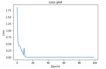

Testing

We have now successfully trained a network using transfer learning to identify images of tanga, qingqi and rickshaw. Let’s test the network to see if it works well with the unseen data.

1. Use the testing data we separated earlier to make predictions.
2. The network predicts the probability of the image belonging to a class.
3. Convert the probabilities into one-hot vectors to assign a vehicle type to the image.
4. Calculate the accuracy of the network on unseen data.

predictions = model.predict(X_test)
predict_vec = np.zeros_like(predictions)
predict_vec[np.arange(len(predictions)), predictions.argmax(1)] = 1
total = 0
true  = 0
for i in range(len(predict_vec)):
if np.sum(abs(np.array(predict_vec[i])- np.array(Y_test[i]))) == 0 :
true += 1
total += 1
accuracy_test = true / total 

We get an accuracy of 91% on the unseen data, which is quite promising, as we only used 216 images for our training. Moreover, we were able to train the network within one minute using a GPU accelerator, while originally the VGG19 model takes a couple of hours to train.

Conclusion

Transfer learning models focus on storing knowledge gained while solving one problem and applying it to a different but related problem. Nowadays, many industries like gaming, healthcare, and autonomous driving are using transfer learning. It would be too early to comment on whether transfer learning is the ultimate solution to the classification problems with small datasets. However, it has surely shown us a direction to move ahead.

Upgrade your data science skillset with our Python for Data Science and Data Science Bootcamp training!