There is so much to explore when it comes to spatial visualization using Python’s Folium library.
Spatial visualization
For problems related to crime mapping, housing prices, or travel route optimization, spatial visualization could be the most resourceful tool for getting a glimpse of how the instances are geographically located. This is beneficial as we are getting massive amounts of data from several sources, such as cellphones, smartwatches, trackers, etc. In this case, patterns and correlations, which otherwise might go unrecognized, can be extracted visually.
This blog will attempt to show you the potential of spatial visualization using the Folium library with Python. This tutorial will give you insights into the most important visualization tools that are extremely useful while analyzing spatial data.
Introduction to folium
Folium is an incredible library that allows you to build Leaflet maps. Using latitude and longitude points, Folium can allow you to create a map of any location in the world. Furthermore, Folium creates interactive maps that may allow you to zoom in and out after the map is rendered.
We’ll get some hands-on practice building a few maps using the Seattle Real-time Fire 911 Calls dataset. This dataset provides Seattle Fire Department 911 dispatches, and every instance of this dataset provides information about the address, location, date/time, and type of emergency of a particular incident. It’s extensive, and we’ll limit the dataset to a few emergency types for the purpose of explanation.
Let’s begin
Folium can be downloaded using the following commands:.
Using pip:
$ pip install folium
Using conda:
$ conda install -c conda-forge folium
Start by importing the required libraries.
import pandas as pd
import numpy as np
import folium
Let us now create an object named ‘seattle_map’ which is defined as a folium.Map object. We can add other folium objects on top of the folium.Map to improve the map rendered. The map has been centered to the longitude and latitude points in the location parameters. The zoom parameter sets the magnification level for the map that’s going to be rendered. Moreover, we have also set the tiles parameter to ‘OpenStreetMap’ which is the default tile for this parameter. You can explore more tiles such as StamenTerrain or Mapbox Control in Folium‘s documentation.
seattle_map = folium. Map
(location = [47.6062, -122.3321],
tiles = 'OpenStreetMap',
 zoom_start = 11)
seattle_map
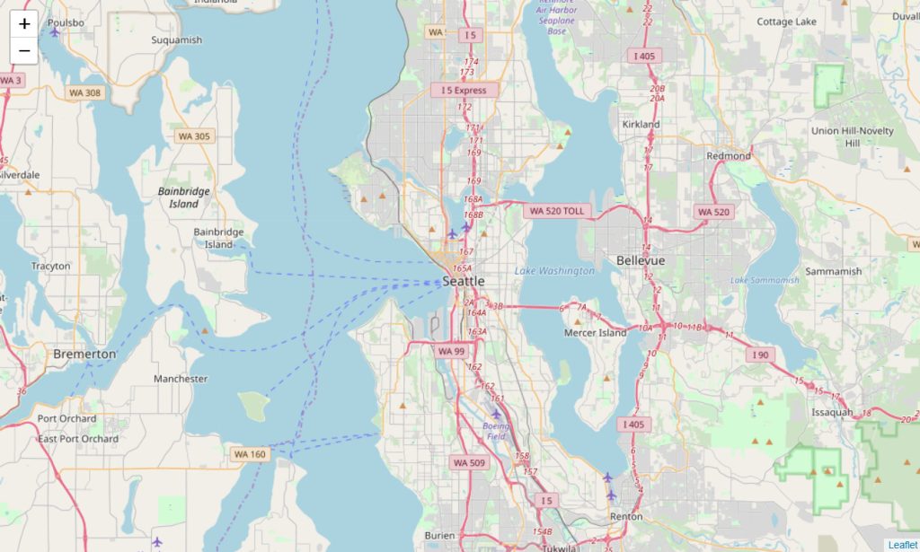
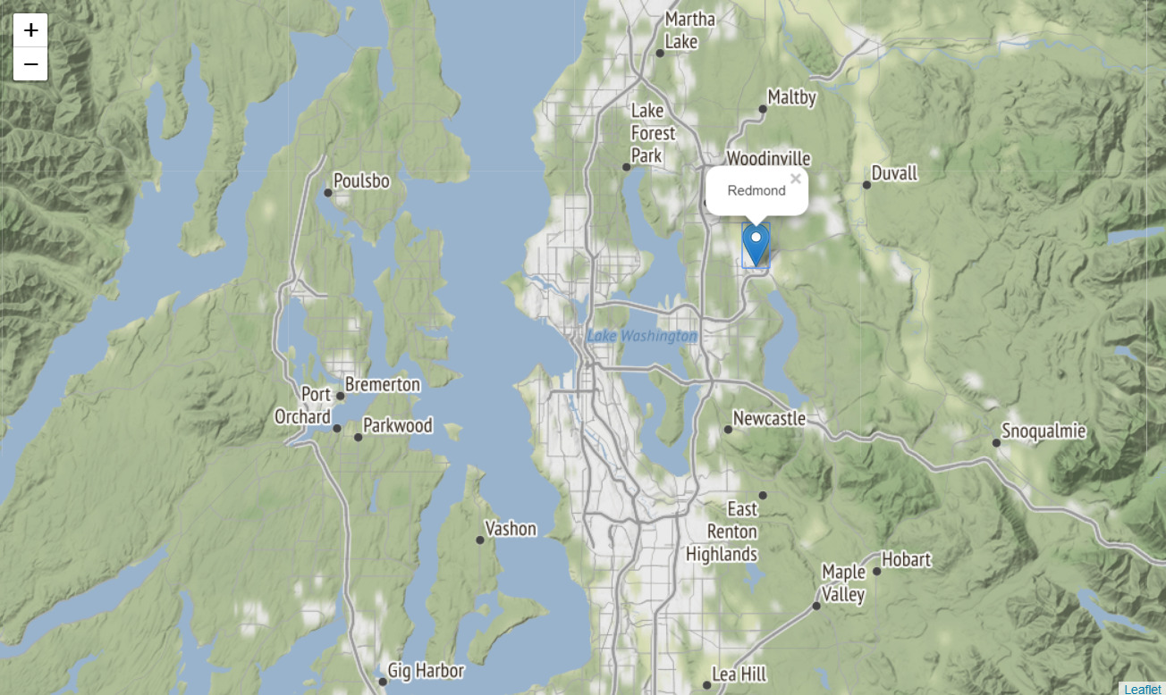
We can observe the map rendered above. Let’s create another map object with a different tile and zoom_level. Through the ‘Stamen Terrain’ tile, we can visualize the terrain data, which can be used for several important applications.
We’ve also inserted a folium. Marker to our ‘seattle_map2’ map object below. The marker can be placed at any location specified in the square brackets. The string mentioned in the popup parameter will be displayed once the marker is clicked, as shown below.
seattle_map2 = folium. Map
(location=[47.6062, -122.3321],
    tiles = 'Stamen Terrain',
    zoom_start = 10)
#inserting marker
folium.Marker(
    [47.6740, -122.1215],
    popup = 'Redmond'
).add_to(seattle_map2)
seattle_map2
We are interested to use the Seattle 911 calls dataset to visualize the 911 calls in the year 2019 only. We are also limiting the emergency types to 3 specific emergencies that took place during this time.
We will now import our dataset, which is available through this link (in CSV format). The dataset is huge, therefore, we’ll only import the first 10,000 rows using the Pandasread_csv method. We’ll use the head method to display the first 5 rows.
(This process will take some time because the data-set is huge. Alternatively, you can download it to your local machine and then insert the file path below)
path = "https://data.seattle.gov/api/views/kzjm-xkqj/rows.csv?accessType=DOWNLOAD"
seattle911 = pd.read_csv(path, nrows = 10000)
seattle911.head()

Using the code below, we’ll convert the datatype of our Datetime variable to Date-time format and extract the year, removing all other instances that occurred before 2019.
seattle911['Datetime'] = pd.to_datetime(seattle911['Datetime'],
                                        format='%m/%d/%Y %H:%M', utc=True)
seattle911['Year'] = pd.DatetimeIndex(seattle911['Datetime']).year
seattle911 = seattle911[seattle911.Year == 2019]
We’ll now limit the Emergency type to ‘Aid Response Yellow’, ‘Auto Fire Alarm’ and ‘MVI – Motor Vehicle Incident’. The remaining instances will be removed from the ‘seattle911’ dataframe.
seattle911 = seattle911[seattle911.Type.isin(['Aid Response Yellow',
                                              'Auto Fire Alarm',
                                              'MVI - Motor Vehicle Incident'])]
We’ll remove any instance that has a missing longitude or latitude coordinate. Without these values, the particular instance cannot be visualized and will cause an error while rendering.
#drop rows with missing latitude/longitude values
seattle911.dropna(subset = ['Longitude', 'Latitude'], inplace = True)

seattle911.head()
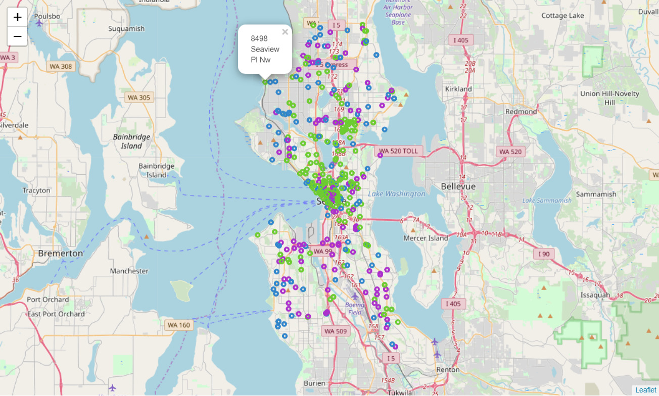
Now let’s step towards the most interesting part. We’ll map all the instances onto the map object we created above, ‘seattle_map’. Using the code below, we’ll loop over all our instances up to the length of the dataframe. Following this, we will create a folium.CircleMarker (which is similar to the folium.Marker we added above). We’ll assign the latitude and longitude coordinates to the location parameter for each instance. The radius of the circle has been assigned to 3, whereas the popup will display the address of the particular instance.
As you can notice, the color of the circle depends on the emergency type. We will now render our map.
for i in range(len(seattle911)):

    folium.CircleMarker( location = [seattle911.Latitude.iloc[i], seattle911.Longitude.iloc[i]],
        radius = 3,
        popup = seattle911.Address.iloc[i],
        color = '#3186cc' if seattle911.Type.iloc[i] == 'Aid Response Yellow' else '#6ccc31'
        if seattle911.Type.iloc[i] =='Auto Fire Alarm' else '#ac31cc',).add_to(seattle_map)
seattle_map
Advanced features provided by folium
Let us now move towards the slightly advanced features provided by Folium. For this, we will use the National Obesity by State dataset which is also hosted on data.gov. There are 2 types of files we’ll be using, a csv file containing the list of all states and the percentage of obesity in each state, and a geojson file (based on JSON) that contains geographical features in form of polygons.
Before using our dataset, we’ll create a new folium.map object with location parameters including coordinates to center the US on the map, whereas, we’ve set the ‘zoom_start’ level to 4 to visualize all the states.
usa_map = folium.Map(
    location=[37.0902, -95.7129],
    tiles = 'Mapbox Bright',
    zoom_start = 4)
usa_map
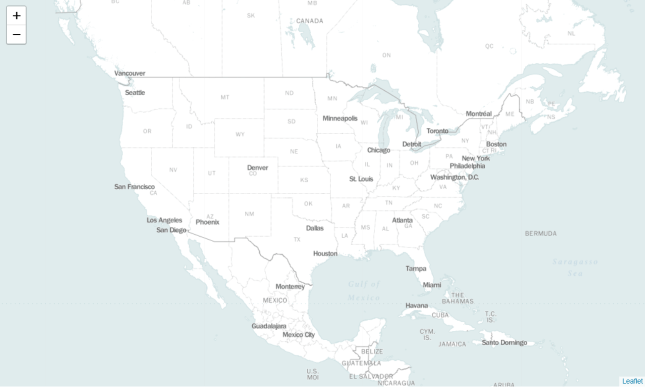
We will assign the URLs of our datasets to ‘obesity_link’ and ‘state_boundaries’ variables, respectively.
obesity_link = 'http://data-lakecountyil.opendata.arcgis.com/datasets/3e0c1eb04e5c48b3be9040b0589d3ccf_8.csv'
state_boundaries = 'http://data-lakecountyil.opendata.arcgis.com/datasets/3e0c1eb04e5c48b3be9040b0589d3ccf_8.geojson'
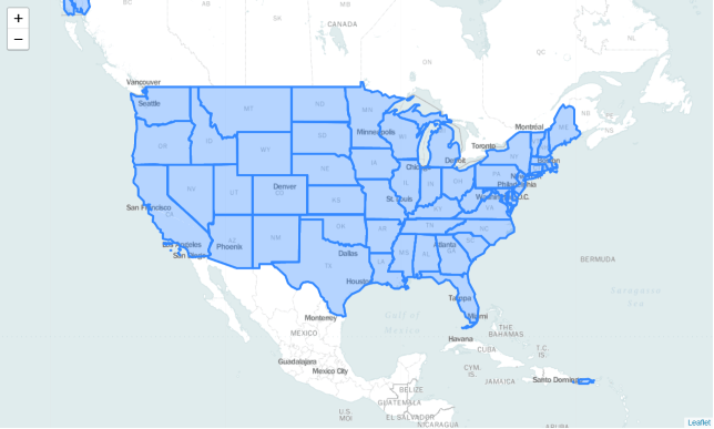
We will use the ‘state_boundaries’ file to visualize the boundaries and areas covered by each state on our folium.Map object. This is an overlay on our original map and similarly, we can visualize multiple layers on the same map. This overlay will assist us in creating our choropleth map that is discussed ahead.
folium.GeoJson(state_boundaries).add_to(usa_map)
usa_map
The ‘obesity_data’ dataframe can be viewed below. It contains 5 variables. However, for the purpose of this demonstration, we are only concerned with the ‘NAME’ and ‘Obesity’ attributes.
obesity_data = pd.read_csv(obesity_link)
obesity_data.head()
Choropleth map
Now comes the most interesting part! Creating a choropleth map. We’ll bind the ‘obesity_data’ data frame with our ‘state_boundaries’ geojson file. We have assigned both the data files to our variables ‘data’ and ‘geo_data’ respectively. The columns parameter indicates which DataFrame columns to use, whereas, the key_on parameter indicates the layer in the GeoJSON on which to key the data.
We have additionally specified several other parameters that will define the color scheme we’re going to use. Colors are generated from Color Brewer’s sequential palettes.
By default, linear binning is used between the min and the max of the values. Custom binning can be achieved with the bins parameter.
folium. Choropleth( geo_data = state_boundaries,
    name = 'choropleth',
    data = obesity_data,
    columns = ['NAME', 'Obesity'],
    key_on = 'feature.properties.NAME',
    fill_color = 'YlOrRd',
    fill_opacity = 0.9,
    line_opacity = 0.5,
    legend_name = 'Obesity Percentage').add_to(usa_map)
folium.LayerControl().add_to(usa_map)
usa_mapFolium. We can visualize the obesity pattern geographically and uncover patterns not visible before. It also helped us in gaining clarity about the data, more than just simplifying the data itself.You might now feel powerful enough after attaining the skill to visualize spatial data effectively. Go ahead and explore Folium‘s documentation to discover the incredible capabilities that this open-source library has to offer.
Thanks for reading! If you want more datasets to play with, check out this blog post. It consists of 30 free datasets with questions for you to solve.
References:
- Python Visualization Modules
- Python Visualization Quickstart
- Seattle Real time Fire Dataset
- https://catalog.data.gov/dataset/national-obesity-by-state
- National Obesity Dataset
Written by Rahim Rasool

