Long short-term memory (LSTM) models are powerful tools primarily used for processing sequential data, such as time series, weather forecasts, or stock prices. When it comes to LSTM models, a common query associated with it is: How Do I Make an LSTM Model with Multiple Inputs?
Before we dig deeper into the multiple inputs feature, let’s explore the multiple inputs functionality of an LSTM model through some easy-to-understand examples.
Typically, an LSTM model handles sequential data in the shape of a 3D tensor (samples, time steps, features). The feature here is the variable at each time step. An LSTM model is tasked to make predictions based on this sequential data, so it is certainly useful for this model to handle multiple sequential inputs.
Think about a meteorologist who wants to forecast the weather. In a simple setting, the input would perhaps be just the temperature. And while this would do a pretty good job in predicting the temperature, adding in other features such as humidity or wind speed would do a far better job.
Imagine trying to predict tomorrow’s stock prices. You wouldn’t rely on just yesterday’s closing price; you’d consider trends, volatility, and other influencing factors from the past. That’s exactly what long short-term memory (LSTM) models are designed to do – learn from patterns within sequential data to make predictions about what values follow subsequently.
While these examples explain how multiple inputs enhance the performance of an LSTM model, let’s dig deeper into the technical process of the question: How do I Make an LSTM Model with Multiple Inputs?
What is a Long Short-Term Memory (LSTM)?
An LSTM is a specialized type of recurrent neural network (RNN) that can “remember” important information from past time steps while ignoring irrelevant information.
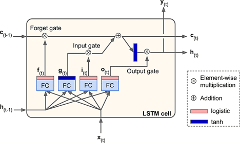
It achieves this through a system of gates as shown in the diagram:
- The input gate decides what new information to store
- The forget gate determines what to discard
- The output gate controls what to send forward
This architecture allows LSTMs to observe relationships between variables in the long term, making them ideal for time-series analysis, natural language processing (NLP), and more.
What makes LSTMs even more impressive is their ability to process multiple inputs. Instead of just relying on one feature, like the closing price of a stock, you can enrich your model with additional inputs like the opening price, trading volume, or even indicators like market sentiment.
Each feature becomes part of a time-step sequence that is fed into the LSTM, allowing it to analyze the combined impact of these multiple factors.
How do I Make an LSTM Model with Multiple Inputs?
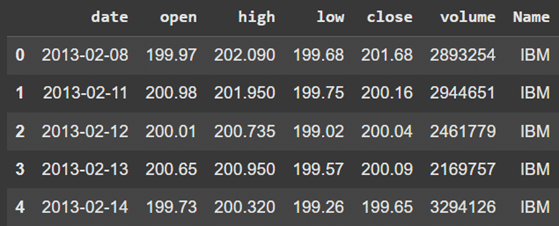
To demonstrate one of the approaches to building an LSTM model with multiple inputs, we can use the S&P 500 Dataset found on Kaggle and focus on the IBM stock data.
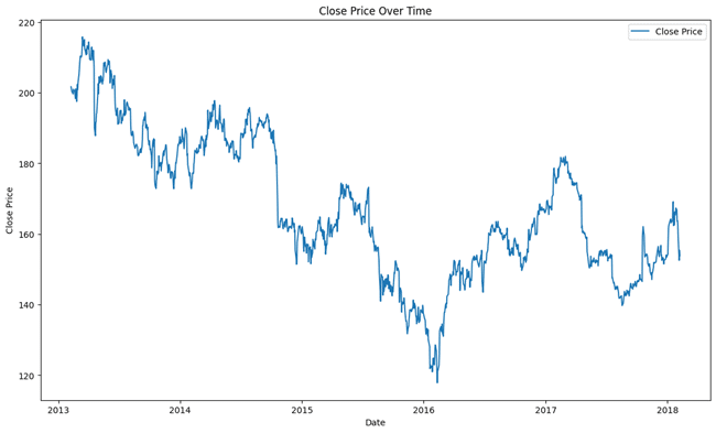
Below is a visualization of the stock’s closing price over time.
The closing price will be the prediction target so understanding the plot helps us contextualize the challenge of predicting the trend. Understanding the intent of adding other inputs to our LSTM model is rather case-specific.
For example, in our case, adding opening price as an additional feature to our LSTM model helps it to capture price swings, reveal market volatility, and most importantly, increased data granularity.
Splitting the Data
Now, we can go ahead and split the data into testing (evaluating) and training (majority of data).
Feature Scaling
To further prepare the data for the LSTM model, we will normalize open and close prices to a range of 0 to 1 to handle varying magnitudes of the two inputs.
Preparing Sequential Data
A key part of training an LSTM is preparing sequential data. The function generates sequences of 60-time steps (offset) to train the model. Here:
- x (Inputs): Sequences of the past 60 days’ features (open and close prices).
- y (Target): The closing price of the 61st day.
For example, X_train has a shape of (947, 60, 2):
- 947: Number of samples.
- 60: Time steps (days).
- 2: Features (open and close prices).
LSTMs require input in the form [samples, time steps, features]. For each input sequence, the model predicts one target value—the closing price for the 61st day. This structure enables the LSTM to capture time-dependent patterns in stock price movements.
The output is presented as follows:
Learning Attention Weights
The attention mechanism further improves the LSTM by assisting it in focusing on the most critical parts of the sequence. It achieves this by learning attention weights (importance of features at each time step) and biases (fine-tuning scores).
These weights are calculated using a softmax function, highlighting the most relevant information and summarizing it into a “context vector.” This vector enables the LSTM to make more accurate predictions by concentrating on the most significant details within the sequence.
Integrating the Attention Layer into the LSTM Model
Now that we have our attention layer, the next step is to integrate it into the LSTM model. The function build_attention_lstm combines all the components to create the final architecture.
- Input Layer: The model starts with an input layer that takes data shaped as [time steps, features]. In our case, that’s [60, 2]—60 time steps and 2 features (open and close prices).
- LSTM Layer: Next is the LSTM layer with 64 units. This layer processes the sequential data and outputs a representation for every time step. We set return_sequences=True so that the attention layer can work with the entire sequence of outputs, not just the final one.
- Attention Layer: The attention layer takes the LSTM’s outputs and focuses on the most relevant time steps. It compresses the sequence into a single vector of size 64, which represents the most significant information from the input sequence.
- Dense Layer: The dense layer is the final step, producing a single prediction (the stock’s closing price) based on the attention layer’s output.
- Compilation: The model is compiled using the Adam optimizer and mean_squared_error loss, making it appropriate for regression tasks like predicting stock prices.
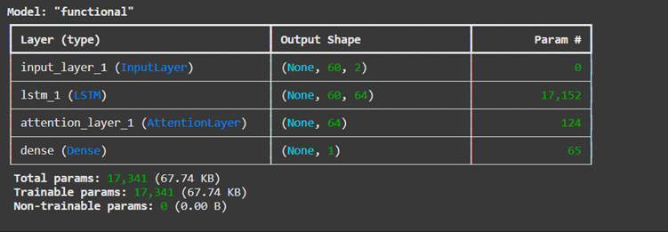
The model summary shows the architecture:
- The LSTM processes sequential data (17,152 parameters to learn).
- The attention layer dynamically focuses on key time steps (124 parameters).
- The dense layer maps the attention’s output to a final prediction (65 parameters).
By integrating attention to the LSTM, this model improves in its ability to predict trends by emphasizing the most important parts of the data sequence.
Building and Summarizing the Model
The output is:
Training the Model
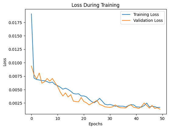
Now that the LSTM model is built, we train it using x_train and y_train. The key training parameters include:
- Epochs: It refers to how many times the model iterates over the training data (can be adjusted to handle overfitting/underfitting)
- Batch size: The model processes 32 samples at a time before updating the weights (smaller batch size takes a longer time but requires less memory)
- Validation data: The model evaluates its performance against the testing set after each iteration
The result of this training process is two metrics:
- Training loss: how well the model fits the training data, and a decreasing training loss shows the model is learning patterns in the training data
- Validation loss: how well the model generalizes unseen data; and if it starts increasing while training loss decreases, it could be a sign of overfitting
Evaluating the Model
The output:
As you can see, the test loss is nearly 0, indicating that the model is performing well and very capable of predicting unseen data.
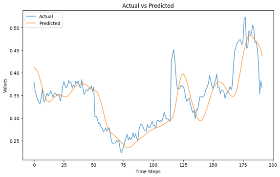
Finally, we have a visual representation of the predicted values vs the actual values of the closing prices based on the testing set. As you can see, the predicted values closely followed the actual values, meaning the model captures the patterns in the data effectively. There are spikes in the actual values which are generally hard to predict due to the nature of time-series models.
Now that you’ve seen how to build and train an LSTM model with multiple inputs, why not experiment further? Try using a different dataset, additional features, or tweaking model parameters to improve performance.
If you’re eager to dive into the world of LLMs and their applications, consider joining the Data Science Dojo’s LLM Bootcamp.


