Naive Bayes, one of the most common algorithms, can do a fairly good job at most classification tasks.
A deep dive into Naïve Bayes for text classification
Often used for classifying text into categories, Naive Bayes uses probability to make predictions for the purpose of classification.
In part 2 of this two-part series, we will dive deep into the underlying probability of Naïve Bayes. In part 1, we delved into the theory of Naïve Bayes and the steps in building a model, using an example of classifying text into positive and negative sentiment.
Now that you have a basic understanding of the probabilistic calculations needed to train a Naive Bayes model and have used it to predict a probability for a given test sentence in part 1, let’s dig deeper into the probability details.
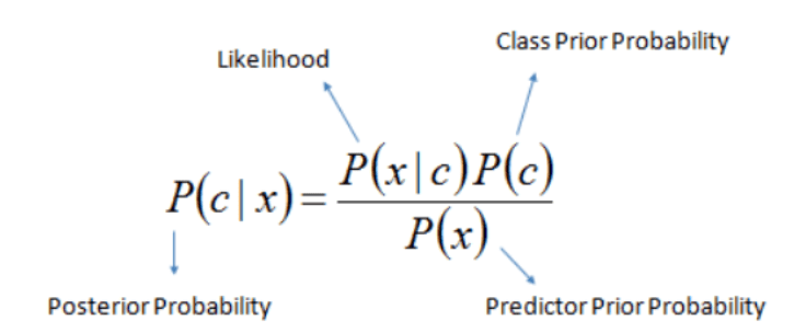
When doing the calculations of probability of the given test sentence in the above section, we did nothing but implement the given probabilistic formula for our prediction at test time:
Decoding
the above mathematical equation:
- “|” = a state which has already been given/or some filtering criteria
- “c” = class/category
- “x” = test example/test sentence
p(c|x) is given the test example x, what is the probability of it belonging to class c? This is also known as posterior probability. This conditional probability is found for the given test example x for each of the training classes.
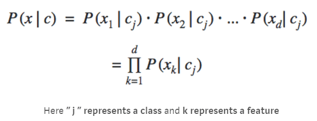
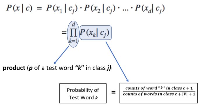
p(x|c) is given the class c, what is the probability of example x belonging to class c? This is also known as the likelihood as it implies how likely example x belongs to class c. This is finding the conditional probability of x out of total instances of class c only – i.e. we have restricted/conditioned our search space to class c while finding the probability of x. We calculate this probability using the counts of words that are determined during the training phase.
We implicitly used this formula twice above in the calculations sections as we had two classes. Do you remember finding the numerical value of product (p of a test word “j” in class c)?
p implies the probability of class c.
This is also known as the prior probability or unconditional probability. We calculated this above in the probability calculations sections (see Step #1 – finding value of term:
p of class c).
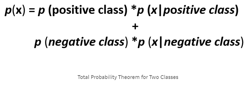
p(x) is known as a normalizing constant so that the probability p(c|x) does actually fall in the range of 0 to 1. So if you remove this, the probability p(c|x) may not necessarily fall in the range of 0 to 1. Intuitively this means the probability of example x under any circumstances or irrespective of its class labels (i.e. whether sentiment is positive or negative).
This is also reflected in total probability theorem, which is used to calculate p(x). The theorem dictates that to find p(x), we will find its probability in all classes (because it is unconditional probability) and simply add them:
This implies that if we have two classes then we would have two terms (in our case, positive and negative sentiments):
Did we use it in the above calculations? No, we did not. Why??? Because we are comparing probabilities of positive and negative classes and the denominator remains the same. So, in this particular case, omitting out the same denominator doesn’t affect the prediction by our trained model. It simply cancels out for both classes. We can include it, but there is no such logical reason to do so. But again, as we have eliminated the normalization constant, the probability p(c|x) may not necessarily fall in the range [0,1].
Avoiding the common pitfalls of the underflow error
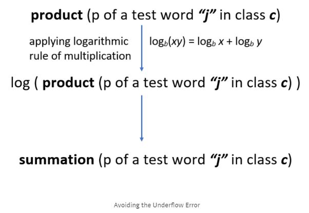
If you noticed, the numerical values of the probabilities of words (i.e. p of a test word “j” in class c) were quite small. Therefore, multiplying all these tiny probabilities to find product (p of a test word “j” in class c) will yield even smaller numerical value. This often results in underflow, which means that for the given test sentence, the trained model will fail to predict its category/sentiment. To avoid this underflow error, we get help from using a mathematical log as follows:
Now instead of multiplication of the tiny individual word probabilities, we will simply add them. And why only log? Why not any other function? Because log increases or decreases monotonically so that it will not affect the order of probabilities. Smaller
probabilities will still stay smaller after the log has been applied on them and vice versa. Let’s say that a test word “is” has a smaller probability than the test word “happy”. After passing these through, log would increase both of their magnitudes, but
maintain their relative differences so that “is” would still have a smaller probability than “happy”. Therefore, without affecting the predictions of our trained model, we can effectively avoid the common pitfall of underflow error.
Concluding notes
Although we live in an age of APIs and practically rarely code from scratch, understanding the algorithmic theory in-depth is extremely vital to develop a sound understanding of how a machine learning algorithm actually works. It is this understanding that differentiates a true data scientist from a naive one and what really matters when training a really good model. So before using out-of-the-box APIs, I personally believe that a true data scientist should code from scratch to really learn the mechanism behind the numbers and the reason why a particular algorithm is better than another for a given task.
One of the best characteristics of the Naive Bayes technique is that you can improve its accuracy by simply updating it with new vocabulary words instead of always retraining it. You will just need to add words to the vocabulary and update the words counts accordingly. That’s it!
This blog was originally published on towardsdatascience.com.
Written by Aisha Jawed


