

Every transformer model ever built shares the same assumption at its core: the best way to move information from one layer to the next is a simple addition, where every layer contributes equally. Layer 1 contributes. Layer 20 contributes. Layer 50 contributes. Each one gets the same fixed weight of 1. This assumption has been baked into transformer design since 2015 and rarely questioned. Kimi AI’s recent technical report on attention residuals questions it, fixes it, and shows consistent performance gains across every benchmark they tested.
This post breaks down what the problem is, how attention residuals solve it, and what the engineering tradeoffs look like at scale.
What Residual Connections Actually Do in Transformers
To understand why attention residuals matter, you need a clear picture of what standard residual connections are doing in the first place, because they serve two distinct purposes and most explanations only cover one of them.
The first purpose is keeping training stable. When you train a deep network, the learning signal (called a gradient) has to travel backwards from the output all the way to the earliest layers. Without a shortcut path, that signal either fades to nothing or grows uncontrollably as it passes through each layer. Residual connections solve this by providing a direct path that the signal can travel through unchanged, which is why training networks with 50+ layers became practical after they were introduced.
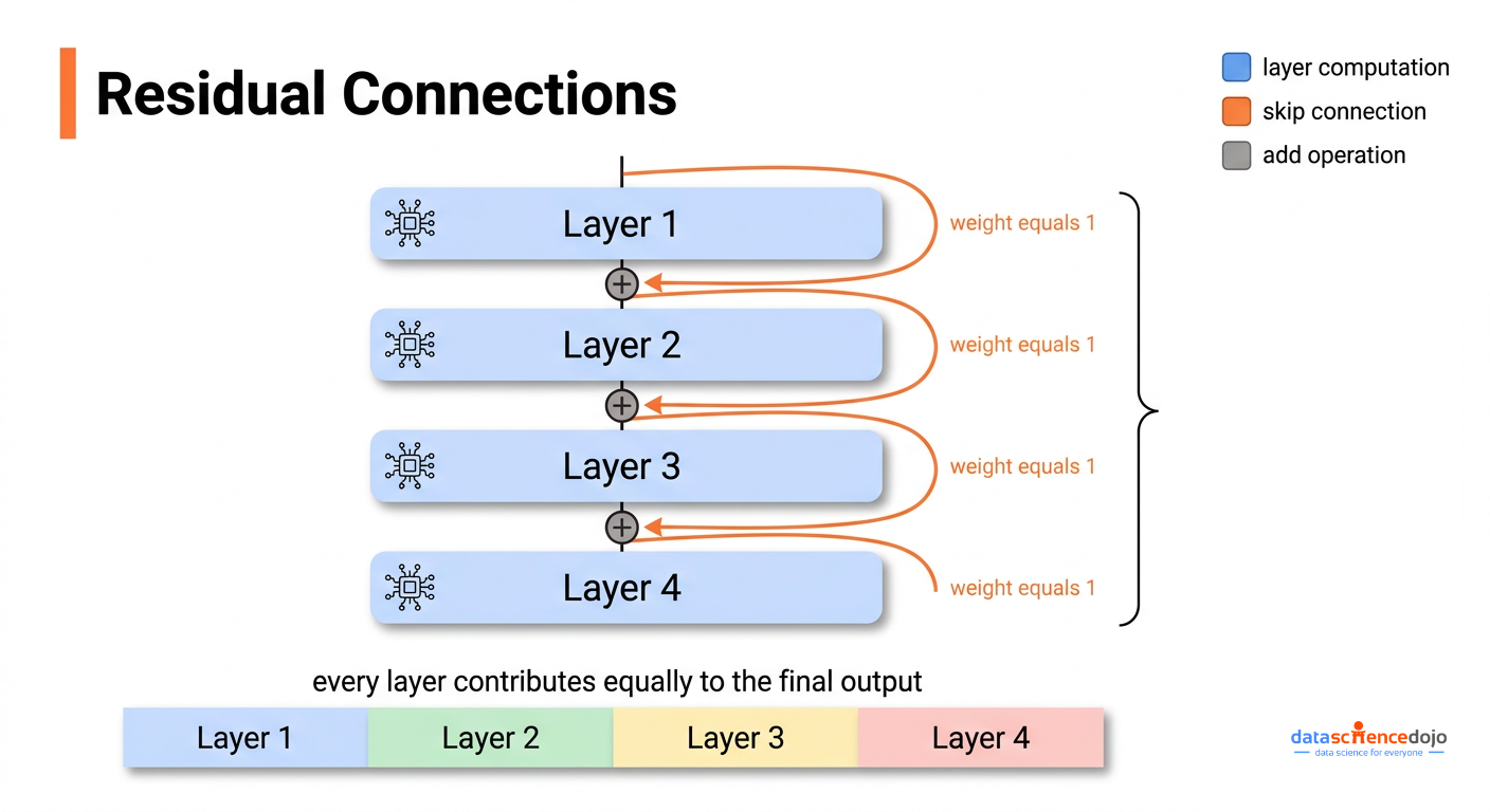
The second purpose, much less discussed, is controlling how information stacks up as it moves through the network. At each layer, the update looks like this:
new hidden state = previous hidden state + what this layer computed
If you trace this across all layers, the value entering any given layer is the original input plus every previous layer’s output, all added together with the same weight of 1. The model has no way to say “I want more of what layer 3 figured out and less of what layer 18 figured out.” Every layer’s contribution is treated as equally important, regardless of what the input actually contains.
Related reading: If you want to revisit how transformers are structured before going deeper here, this primer on transformer architecture covers the core components clearly.
The Hidden State Growth Problem
This equal-weight stacking creates a concrete problem that gets worse the deeper the model gets. It is known as PreNorm dilution, and here is what causes it.
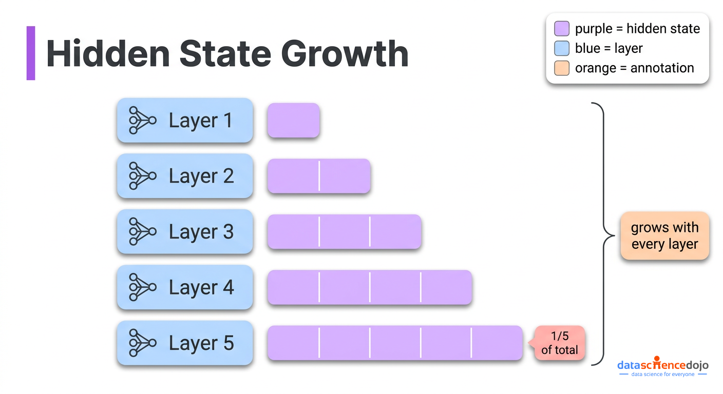
Modern transformers rescale (normalize) the accumulated value before passing it into each layer’s computation. This rescaling became standard because it keeps training stable. The sequence of events at each layer is:
- The accumulated value, the sum of all previous layer outputs stacked together, gets rescaled to a standard size before the new layer processes it
- The layer produces an output at that standard size, roughly the same scale every time
- That output gets added back to the accumulated value, which has not been rescaled
The accumulated value grows with every layer, because you keep adding standard-sized outputs to it. By layer 50, the pile is roughly 50 times larger than a single layer’s output. Layer 50’s own contribution, which is standard-sized, is now just 1/50th of the total pile. Layer 100’s contribution is 1/100th. The model can still technically read individual layer contributions through the rescaling step, but their actual influence on the final result keeps shrinking as the pile grows.
The consequence is not just theoretical. Research has shown that you can remove a significant fraction of layers from standard transformers entirely, and performance barely changes. The model had already learned to largely ignore those layers, because their contributions were too diluted to matter.
The Core Insight: Depth Has the Same Problem That Sequences Did
The reason this paper is worth taking seriously is that it identifies a genuine structural parallel, and that parallel points directly to the solution.
Recurrent neural networks (RNNs), the dominant sequence models before transformers, had an identical problem — just along the sequence dimension rather than the depth dimension. To process word 100 in a sentence, an RNN had to compress everything from words 1 through 99 into a single fixed-size summary. Information from early words got diluted as the sequence grew longer. The transformer architecture solved this by replacing that sequential compression with direct attention: every word can look back at every previous word, with learned weights that depend on the actual content. That shift was what made transformers dramatically better at language tasks.
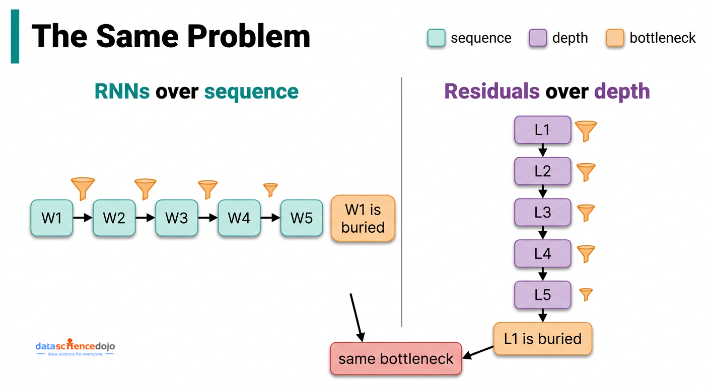
Standard residual connections create the same bottleneck, just oriented differently. Instead of compressing past words into one summary, they compress all previous layer outputs into one growing accumulated value. The information that layer 3 produced cannot be selectively retrieved by layer 40 — it can only be accessed through the blurred total that has been building up between them.
Attention Residuals (AttnRes) apply the transformer’s own solution to this problem, but across layers instead of across words.
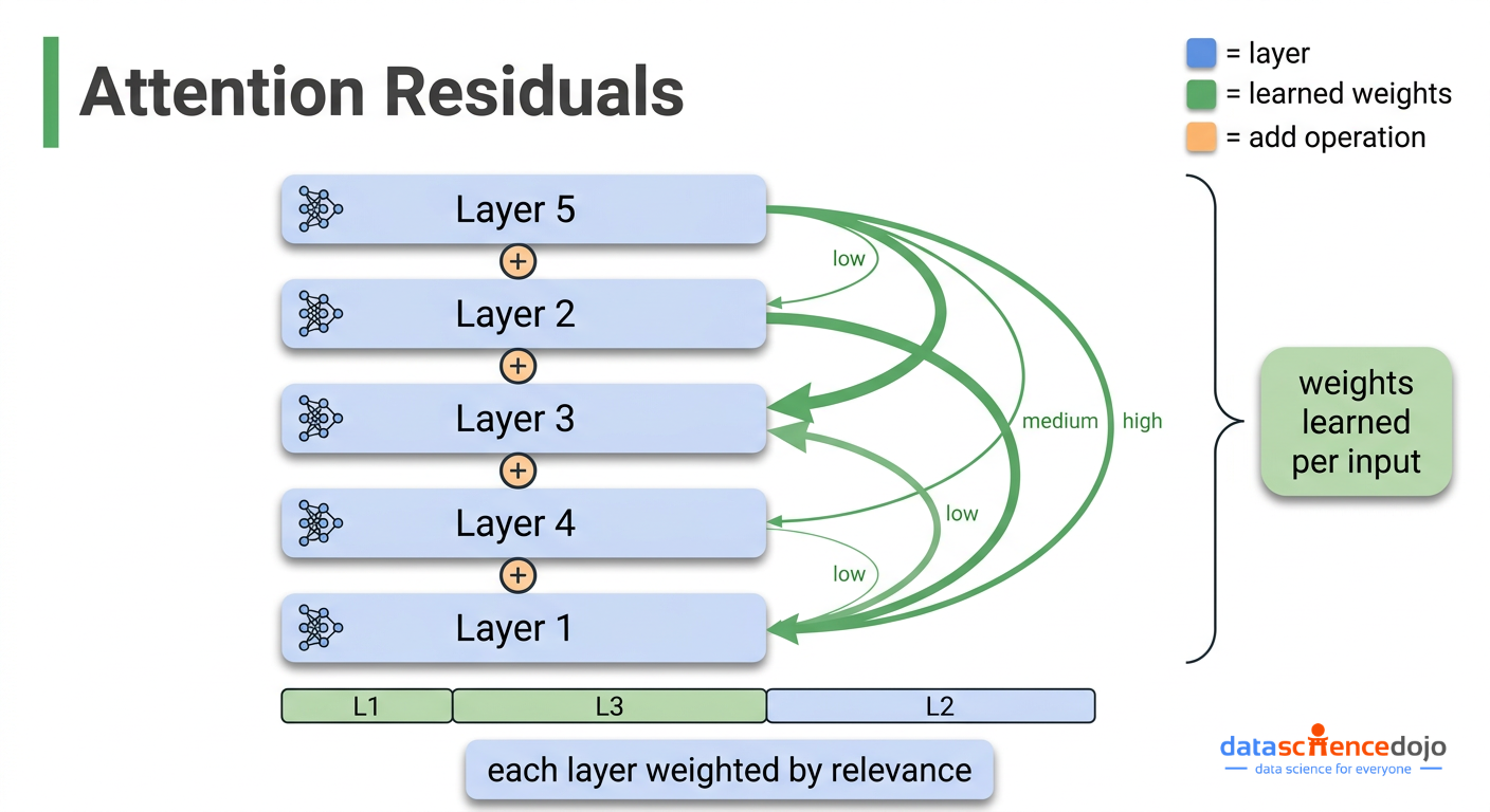
Rather than fixing every layer’s contribution weight at 1, they replace the fixed accumulation with a weighted sum where the weights are learned and depend on the actual input:
new hidden state = weighted sum of all previous layer outputs (weights learned, must sum to 1, vary with input)
Because the weights must sum to 1 (via a softmax operation, which just means they compete with each other and always add up to 100%), if layer 3’s output is highly relevant to what layer 40 is doing, layer 40 can put more weight on layer 3 and less on others. This is selective, content-aware retrieval across layers — the same idea that made attention so effective across words.
Related reading: For context on how attention works across words before connecting it to layers, this breakdown of self-attention is a useful reference.
How Full Attention Residuals Work in Practice
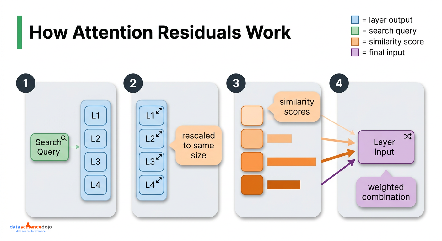
The mechanics for attention residuals are simpler than they might sound. For each layer, the computation works like this:
- Each layer gets one small learned vector. Think of this as the layer’s “search query” — it represents what that layer is looking for from the layers that came before it
- The outputs of all previous layers act as the things being searched over
- Before computing how relevant each previous layer is, each output gets rescaled to a standard size. This prevents a layer that happens to produce unusually large outputs from dominating just because of scale rather than actual relevance
- A similarity score is computed between the search query and each previous layer’s output, and these scores are converted into weights that sum to 1
- The layer’s input is the weighted combination of all previous layer outputs, using those weights
The extra parameters this adds are minimal: one small vector per layer and one rescaling operation per layer. For a 48 billion parameter model, this is a rounding error. One important implementation note: those search query vectors must be initialized to zero at the start of training. This makes Attention Residuals behave exactly like standard residuals at initialization, so training starts stable and the selective weighting develops gradually as the model learns.
In terms of memory during standard training, Full Attention Residuals adds essentially no overhead. The layer outputs it needs are already being kept in memory for the backward pass anyway. The problem appears when you try to train at scale.
The Engineering Problem: Why Full Attention Residuals Does Not Scale Directly
Training large models on GPU clusters requires splitting the work across many machines. Two techniques that make this practical are relevant here:
- Saving memory by recomputing: Rather than storing every intermediate value in memory during the forward pass, you discard them and recompute what you need during the backward pass. This frees up GPU memory at the cost of extra computation.
- Splitting the model across GPUs: Different layers run on different machines. The output of one group of layers gets sent to the next machine to continue the forward pass. This is called pipeline parallelism.
Full AttnRes conflicts with both of these. Each layer needs the outputs of every previous layer, which means those outputs cannot be discarded and recomputed — they must stay in memory the entire time. Under pipeline parallelism, all of those stored outputs also have to be transmitted across machine boundaries at every step. The memory and communication cost grows proportionally to the number of layers times the size of each layer’s output. For a 128-layer model, this becomes impractical.
Block AttnRes: The Practical Solution
Block AttnRes solves this with a compression step. Instead of attending over every individual layer output, you:
- Divide the layers into N groups called blocks (the paper uses N around 8)
- Within each block, use standard residual addition to accumulate layer outputs into one summary vector per block
- Apply learned attention across just those N block-level summaries rather than across all individual layers
- Within the current block, also attend over the partial accumulation of layers completed so far in that block
This brings memory and communication costs down from scaling with the total number of layers to scaling with just the number of blocks. With 128 layers and 8 blocks, you go from needing 128 stored values per token to needing 8. The cross-machine communication cost shrinks by the same factor.
Related reading: This post on distributed training strategies covers how model parallelism and pipeline stages work in more detail if you want the infrastructure context.
The number of blocks N sits between two extremes:
- 1 block reduces to standard residual connections, with just the original input isolated as a separate source
- As many blocks as there are layers recovers Full AttnRes, attending over every individual layer output separately
The ablations show that 2, 4, and 8 blocks all reach nearly identical performance, while larger blocks (16, 32) start degrading back toward the baseline. Eight blocks is chosen as a practical default because it keeps overhead manageable at scale while capturing most of the benefit.
The Two-Phase Computation Strategy
During inference, a naive implementation would redo the full attention computation at every single layer, which is expensive. Kimi AI’s team avoids this with a two-phase approach:
- Phase 1: The search query vectors are learned parameters that do not depend on the current input, so all queries within a block are known upfront. A single batched computation handles the attention across block summaries for all layers in the block at once, reading each block summary once and reusing it rather than reading it separately for each layer.
- Phase 2: The within-block attention is computed sequentially as that block’s partial accumulation builds up, then merged with the Phase 1 results.
The end result is that inference latency overhead stays under 2% on typical workloads, and training overhead stays under 4%.
Related reading: For background on efficient inference techniques, this overview of KV caching and memory optimization is directly relevant to the inference design decisions here.
Results: What the Numbers Actually Show
The paper tests AttnRes across five model sizes, comparing a standard baseline, Full AttnRes, and Block AttnRes with around 8 blocks.
| Benchmark | Baseline | AttnRes | Delta |
|---|---|---|---|
| MMLU | 73.5 | 74.6 | +1.1 |
| GPQA-Diamond | 36.9 | 44.4 | +7.5 |
| BBH | 76.3 | 78.0 | +1.7 |
| Math | 53.5 | 57.1 | +3.6 |
| HumanEval | 59.1 | 62.2 | +3.1 |
| MBPP | 72.0 | 73.9 | +1.9 |
| C-Eval | 79.6 | 82.5 | +2.9 |
The scaling law result is the most significant for anyone thinking about training costs: Block AttnRes matches the performance of a standard baseline that was trained with 1.25x more compute. You get the same model quality for roughly 80% of the training budget, just by changing how layer outputs are combined.
The benchmark gains make sense when you think about what Attention Residuals is actually fixing. The largest improvements are on multi-step reasoning tasks like GPQA-Diamond (+7.5) and Math (+3.6). These are tasks where a later layer needs to selectively build on something a much earlier layer figured out, rather than receiving everything blended together equally. General knowledge recall benchmarks like MMLU show smaller but still consistent gains, which is expected because those tasks depend less on chaining reasoning steps and more on information that was stored during training.
The training dynamics data from the paper is also worth examining. In the standard baseline, each layer’s output magnitude grows steadily with depth, and the learning signal during training is heavily concentrated in the earliest layers. Block AttnRes produces a bounded, repeating pattern in output magnitudes, with the learning signal distributing more evenly across all layers. The structural problem shows up visibly fixed in the training behavior, not just in the final benchmark numbers.
What the Model Actually Learns to Do
One of the more interesting parts of the paper is the visualization of the learned weight distributions, because they reveal that the model does not simply learn to spread attention evenly across everything.
Three consistent patterns emerge from the learned weights:
- Locality is preserved. Each layer still puts its highest weight on the immediately preceding layer, which makes sense because most computation at each layer still depends on what just happened directly before it.
- Selective reach-back connections emerge. Certain layers learn to put meaningful weight on much earlier layers when useful. The original input embedding retains non-trivial weight throughout the full depth of the network, particularly before attention layers.
- Attention layers and MLP layers develop different patterns. Layers before an MLP step concentrate more heavily on recent layers. Layers before an attention step maintain broader reach across the full layer history.
These patterns are not designed in — they emerge from training. Block AttnRes reproduces the same essential structure as Full AttnRes, with sharper and more decisive weights, which suggests that compressing to block summaries acts as a mild form of regularization while preserving the information pathways that actually matter.
Frequently Asked Questions
What is the difference between attention residuals and self-attention?
Standard self-attention is about relationships between words (or tokens) in the input: each word looks at every other word to decide what context is relevant. Attention residuals are about relationships between layers: each layer looks at the outputs of all previous layers to decide what to build on. They are completely separate mechanisms. Attention Residuals changes how layer outputs are combined in the residual stream and has no effect on how the attention heads inside each layer process words.
Does this require retraining from scratch?
Yes. Attention residuals change how information flows through the network at a fundamental level, so they need to be part of training from the start. The learned search query vectors for each layer must be initialized to zero, so the system starts out behaving like standard residuals and gradually develops selective weighting as training progresses.
How does this compare to DenseFormer?
DenseFormer also gives each layer access to all previous layer outputs, but uses fixed weights that are learned once during training and then frozen. The paper’s ablation results are clear: DenseFormer shows no improvement over the baseline (1.767 vs 1.766 validation loss). Having weights that adapt to each input is what produces the gains. Attention residuals tested without input-dependent weights also underperforms (1.749), which confirms that content-aware selection is the key ingredient, not just giving layers access to earlier outputs.
Can this be added to any transformer architecture?
Attention Residuals is designed as a drop-in replacement for standard residual connections. The paper integrates it into a Mixture-of-Experts model (Kimi Linear 48B) without changing the attention heads, feed-forward layers, routing logic, or any other component. In principle it should be compatible with any transformer that uses standard residual connections, which is essentially all of them.
Why approximately 8 blocks specifically?
The paper tests block counts ranging from 1 (equivalent to Full AttnRes) up to 32. Block counts of 2, 4, and 8 all reach nearly identical validation loss, while 16 and 32 start degrading back toward baseline performance. Eight is chosen as the default because it is small enough to keep memory and cross-machine communication manageable during large-scale training while still capturing most of the benefit. As hardware improves, finer-grained blocking becomes more viable.
So What Does This Mean for Engineers Working with LLMs?
If you are building on top of existing models through fine-tuning or running inference, attention residuals do not change anything about your workflow today. The gains come from training, and models that incorporate Attention Residuals will simply perform better on reasoning-heavy tasks out of the box.
If you are training or fine-tuning at scale, the paper’s GitHub repository (linked in the abstract) includes a PyTorch reference implementation. The training overhead is small enough that it is worth evaluating, particularly for workloads where compute efficiency matters.
The more significant implication is architectural. AttnRes changes the optimal balance between depth and width in a model: the paper’s architecture sweep shows that AttnRes benefits from deeper, narrower networks compared to the standard baseline, because it can actually use the additional layers rather than wasting them to dilution. If you are doing any kind of architecture search for a new training run, this shifts what the optimal configuration looks like.
Read next: Understanding scaling laws and compute-optimal training gives the framework for thinking about where the 1.25x compute equivalence result fits in the broader picture of model efficiency research.
Conclusion
The standard residual connection has been a fixed assumption in transformer design for a decade. Attention residuals do not throw it out — they generalize it, replacing a fixed equal-weight accumulation with a learned, input-dependent weighted sum over all previous layer outputs. The mechanism adds minimal parameters (one small vector and one rescaling operation per layer), works with existing architectures, and produces consistent gains across model sizes and tasks.
Block AttnRes makes this practical at scale by compressing layer history into block-level summaries, keeping training overhead under 4% and inference overhead under 2%. The engineering work around incremental cross-machine communication and the two-phase computation strategy is what turns a theoretically sound idea into something that actually runs efficiently on a distributed training cluster.
The paper is available on arXiv and the implementation is on GitHub. For engineers working on LLM training pipelines, it is a concrete and well-evidenced architectural improvement worth understanding now.